# Single-Cell Proteomics Analysis with `scp` {#sec-appendix-scp .unnumbered}
## Learning Objectives
By the end of this appendix you will be able to:
- Identify the key analytical challenges that distinguish single-cell proteomics (SCP) from bulk proteomics
- Describe how the `scp` package extends `QFeatures` with `SingleCellExperiment` assays
- Load and inspect an SCP dataset from `scpdata`
- Perform cell-level quality control and annotation audit
- Filter PSMs and aggregate to peptide- and protein-level quantification
- Normalize and assess batch structure in SCP data
- Conduct or cross-reference statistical methods for differential abundance in SCP
## What Changes from Bulk Proteomics
### Low Input and Identification Sparsity
Single-cell proteomics starts with picogram amounts of protein per cell — orders of magnitude less than a typical bulk proteomics experiment. The immediate consequence is **identification sparsity**: a bulk TMT experiment may quantify 6000–8000 proteins per sample, while a single cell typically yields 1000–3000 identified proteins. Many peptides that are present are not detected in every cell, producing a high proportion of missing values that follows a structure-dependent pattern rather than a purely random one.
::: {.callout-warning title="Sparsity is not a bug"}
Do not treat SCP missingness as a universal property. The fraction of missing values depends on the acquisition method (TMT, label-free, diaPASEF), the instrument, the carrier-channel strategy, and the depth of the fractionation. Always report the detection rate and missingness pattern for your specific dataset.
:::
### Batch and Acquisition Structure
Most SCP experiments use multiplexed acquisition (TMT, TMTpro, or similar isobaric labels) to measure multiple single cells simultaneously. A typical design places each cell in one TMT channel, includes a **carrier channel** (100–200 cell-equivalents of peptide) to boost identification, and often a **reference channel** (a pool of all samples) for normalization across batches. Several TMT runs are combined into an experiment, so the data has a nested structure:
- **Cells** are the biological unit (individual cells loaded into channels)
- **Channels** are the TMT reporter-ion slots within a single run
- **Acquisition runs** (also called batches) group a set of channels measured together
- **Biological replicates** are independent cell populations; a single experiment may have only technical replication at the cell level
::: {.callout-note title="Distinguishing levels of replication"}
A 16-plex TMTpro run with 14 single cells, one carrier, and one reference channel provides 14 technical replicates of the cell type, not 14 biological replicates. True biological replication requires cells from independent cultures, organisms, or tissue samples. State your replication structure explicitly in any SCP analysis.
:::
### Carrier and Reference Channels
The **carrier (or booster) channel** is a distinctive feature of TMT-based SCP. It contains a relatively large amount of peptide (often 50–200 cell-equivalents) from the same cell type. During MS acquisition, the carrier boosts the precursor intensity, improving the chance that low-abundance single-cell peptides are selected for fragmentation and identification. The carrier's reporter ion signal is usually an order of magnitude higher than the single-cell channels and is excluded from downstream quantification.
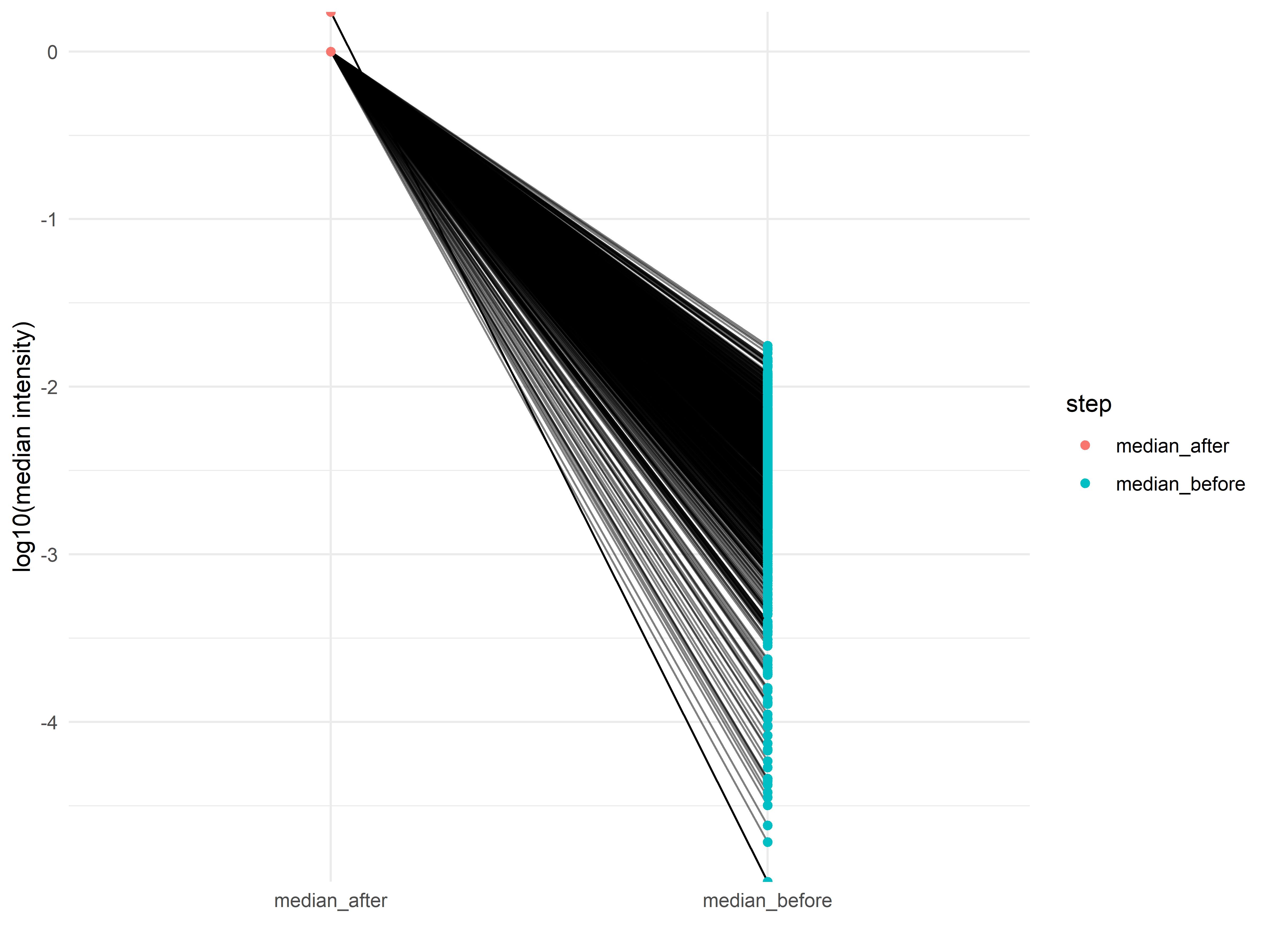
The **reference channel** (a pooled sample from all conditions) provides a common anchor across batches. After median normalization, each single-cell channel within a run is scaled so that the reference channel has the same median intensity across runs, enabling between-run comparison.
## The `scp` Data Model
The `scp` package builds on the `QFeatures` container (Chapter 5) to represent the multi-level structure of SCP data. Each **acquisition run** (a single TMT experiment) is stored as one `assay` in the `QFeatures` object:
- Each assay is a `SingleCellExperiment` (SCE) object, which extends `SummarizedExperiment` with methods designed for single-cell data
- **Columns** of the SCE correspond to **channels** (individual cell samples, plus carrier and reference channels)
- **Rows** correspond to **identified PSMs** (in the raw assays) or to peptides/proteins (in aggregated assays)
- **`colData`** stores channel-level metadata: the cell annotation, the acquisition run, the TMT channel index, and quality metrics
- **`rowData`** stores feature-level identification information: peptide sequence, protein accession, search score, posterior error probability (PEP), and any decoy/contaminant flags
Multiple acquisition runs are kept as separate assays until they are joined (via `joinAssays()`) for a combined analysis. The aggregation functions `aggregateFeatures()` from `QFeatures` collapse PSMs first to peptides and then to proteins, each step producing a new `SingleCellExperiment` assay within the same `QFeatures` container.
```
QFeatures object
├── Assay 1: single_cell_psms (SCE)   ← PSM-level, one per run
├── Assay 2: single_cell_psms_2 (SCE) ← PSM-level, run 2
├── ...
├── joined_psms (SCE)                  ← all runs joined
├── peptides (SCE)                     ← aggregated PSMs → peptides
└── proteins (SCE)                     ← aggregated peptides → proteins
```
This hierarchical structure lets each step of the workflow — filtering, normalization, aggregation, and modeling — operate at the appropriate level while preserving the provenance of each quantitative value.
## Import and Inspection
We use the `leduc2022` dataset from `scpdata` for this appendix. This is a TMTpro-16 experiment profiling the proteome of naive, primed, and naive-reset pluripotent stem cell states [@leduc2022pluripotent]. It was chosen because it represents a single 16-plex run, making it compact enough for routine book rendering while illustrating the core SCP workflow. The full dataset includes a carrier channel and a reference channel alongside single-cell channels from three pluripotency conditions.
::: {.callout-note title="Dataset rationale"}
`leduc2022` is a single-run TMTpro-16 experiment, so it avoids the complexity of multi-run joining while preserving all essential SCP features: carrier channel, reference channel, and cell-level annotation with condition labels. If your computer has limited memory, further subset the PSM table by removing the carrier channel rows before aggregation; the code below demonstrates this.
:::
```{r}
#| eval: true
#| message: true
library(scp)
library(scpdata)
library(scater)
library(ggplot2)
library(dplyr)
library(tidyr)
library(patchwork)
```
```{r}
#| eval: true
#| message: true
# Load the leduc2022 dataset
leduc <- leduc2022()
leduc
```
Inspect the available assays and their dimensions:
```{r}
#| eval: true
names(leduc)
```
```{r}
#| eval: true
dims(leduc)
```
```{r}
#| eval: true
# Inspect column metadata
colData(leduc) |> head()
```
```{r}
#| eval: true
# Inspect row metadata of the PSM-level assay
rowData(leduc[[1]]) |>
    as.data.frame() |>
    select(Sequence, Proteins, Reverse, Potential.contaminant, PEP, Score) |>
    head()
```
```{r}
#| eval: true
# Table of cell types / conditions represented
colData(leduc)$SampleType |> table()
```
The output confirms the presence of single-cell channels, a carrier channel, and a reference channel. The `colData` contains the annotation we need for downstream analysis: the cell condition (SampleType), the TMT channel, and the acquisition run.
::: {.callout-note title="Subsetting for memory-constrained rendering"}
If the full PSM table causes memory issues during book rendering, subset the dataset to exclude the carrier channel and keep only the single-cell channels before aggregation:
```{r}
leduc <- subsetByColData(leduc,
    colData(leduc)$SampleType != "Carrier")
```
This removes the high-intensity carrier channel that contributes many PSM identifications but is not part of the quantitative comparison.
:::
## Cell Annotation Audit and Quality Control
We compute per-channel quality metrics directly from the PSM-level assay:
```{r}
#| eval: true
# Number of PSMs identified per channel (non-NA quantifications)
n_psms <- colSums(!is.na(assay(leduc[[1]])))
nFeatures <- data.frame(
    leduc2022_psms = n_psms,
    row.names = names(n_psms)
)
names(nFeatures)
```
```{r}
#| eval: true
head(nFeatures)
```
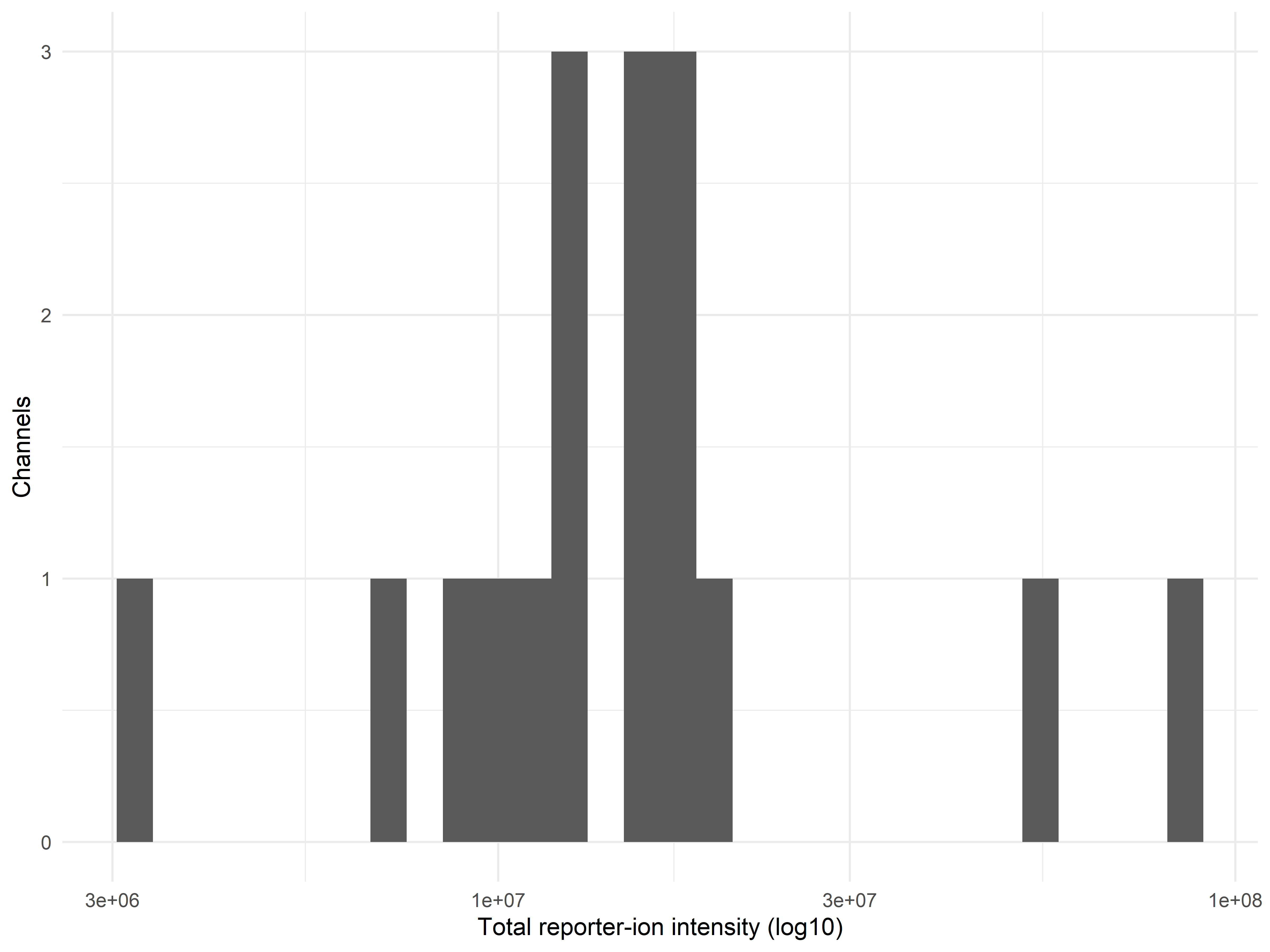
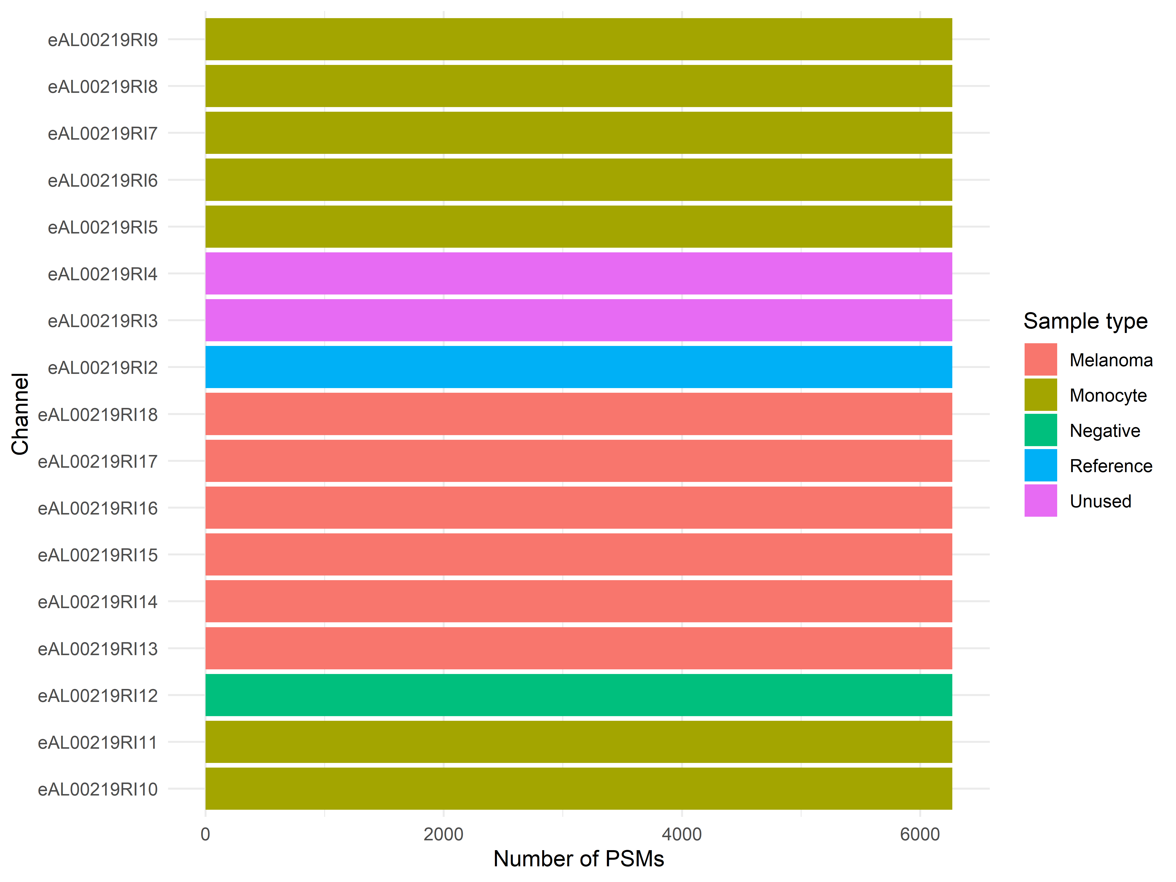
These metrics help flag problematic channels: channels with very few identifications, abnormally low total intensity, or unusual missingness patterns.
```{r}
#| eval: true
#| fig-cap: "QC metrics per channel: number of identified PSMs and total intensity."
# Visualise per-channel identification counts
nPSM_data <- nFeatures |>
    tibble::rownames_to_column("channel") |>
    left_join(
        colData(leduc) |>
            as.data.frame() |>
            tibble::rownames_to_column("channel"),
        by = "channel"
    )

p1 <- ggplot(nPSM_data, aes(x = reorder(channel, leduc2022_psms), y = leduc2022_psms, fill = SampleType)) +
    geom_col() +
    coord_flip() +
    labs(x = "Channel", y = "Number of PSMs", fill = "Sample type") +
    theme_minimal()

# Total intensity per channel
qplot(colSums(assay(leduc[[1]]), na.rm = TRUE)) +
    labs(x = "Total reporter-ion intensity (log10)", y = "Channels") +
    scale_x_log10() +
    theme_minimal()
p1
```
Carrier channels should show substantially higher intensity and more identifications. If a single-cell channel approaches carrier-level intensity, it may indicate a doublet (two cells in one channel). Conversely, channels with very low counts may represent empty channels or failed labeling.
```{r}
#| eval: true
#| fig-cap: "Missing value proportion per channel."
# Proportion of missing values per column
pct_missing <- apply(assay(leduc[[1]]), 2, function(x) mean(is.na(x))) * 100
qplot(pct_missing, bins = 15) +
    labs(x = "Missing PSMs (%)", y = "Number of channels") +
    theme_minimal()
```
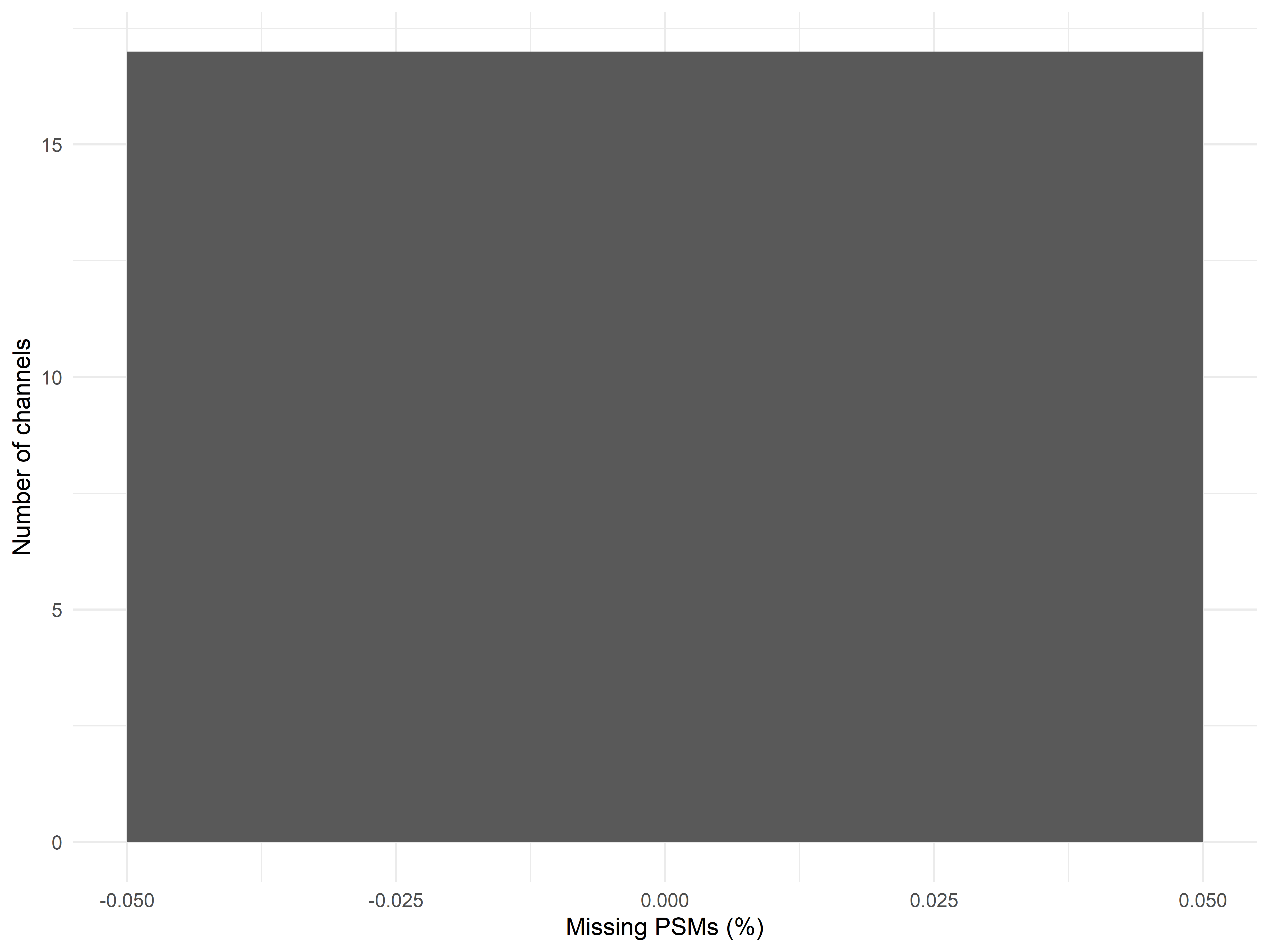
::: {.callout-warning title="Do not impute SCP data with bulk methods"}
Bulk-proteomics imputation methods (Chapter 18), especially those designed for MCAR/MAR mechanisms, assume a relatively low proportion of missing values distributed across features. SCP data routinely exceeds 40–60 % missing values, and the missingness is driven by the stochastic nature of precursor selection in data-dependent acquisition (DDA). Bulk-style imputation under these conditions can introduce severe bias. Filter features with excessive missingness instead, and consider specialized SCP imputation approaches only after careful evaluation.
:::
## Filtering and Aggregation from PSMs to Proteins
### PSM-Level Filtering
Before aggregation, remove common artefactual identifications:
```{r}
#| eval: true
cat("PSMs before filtering:", nrow(leduc[[1]]), "\n")
leduc <- filterFeatures(leduc,
    i = 1,
    ~ Reverse != "+" &
        Potential.contaminant != "+" &
        PEP < 0.05)

cat("PSMs after filtering:", nrow(leduc[[1]]), "\n")
```
Optional: remove the carrier channel from the quantitative assays, keeping only single-cell and reference channels:
```{r}
#| eval: true
# Remove carrier channel (high-intensity booster not used in quant comparison)
leduc <- subsetByColData(leduc,
    colData(leduc)$SampleType != "Carrier")

cat("Channels after carrier removal:", ncol(leduc[[1]]), "\n")
colData(leduc)$SampleType |> table()
```
### Aggregation: PSM to Peptide, Peptide to Protein
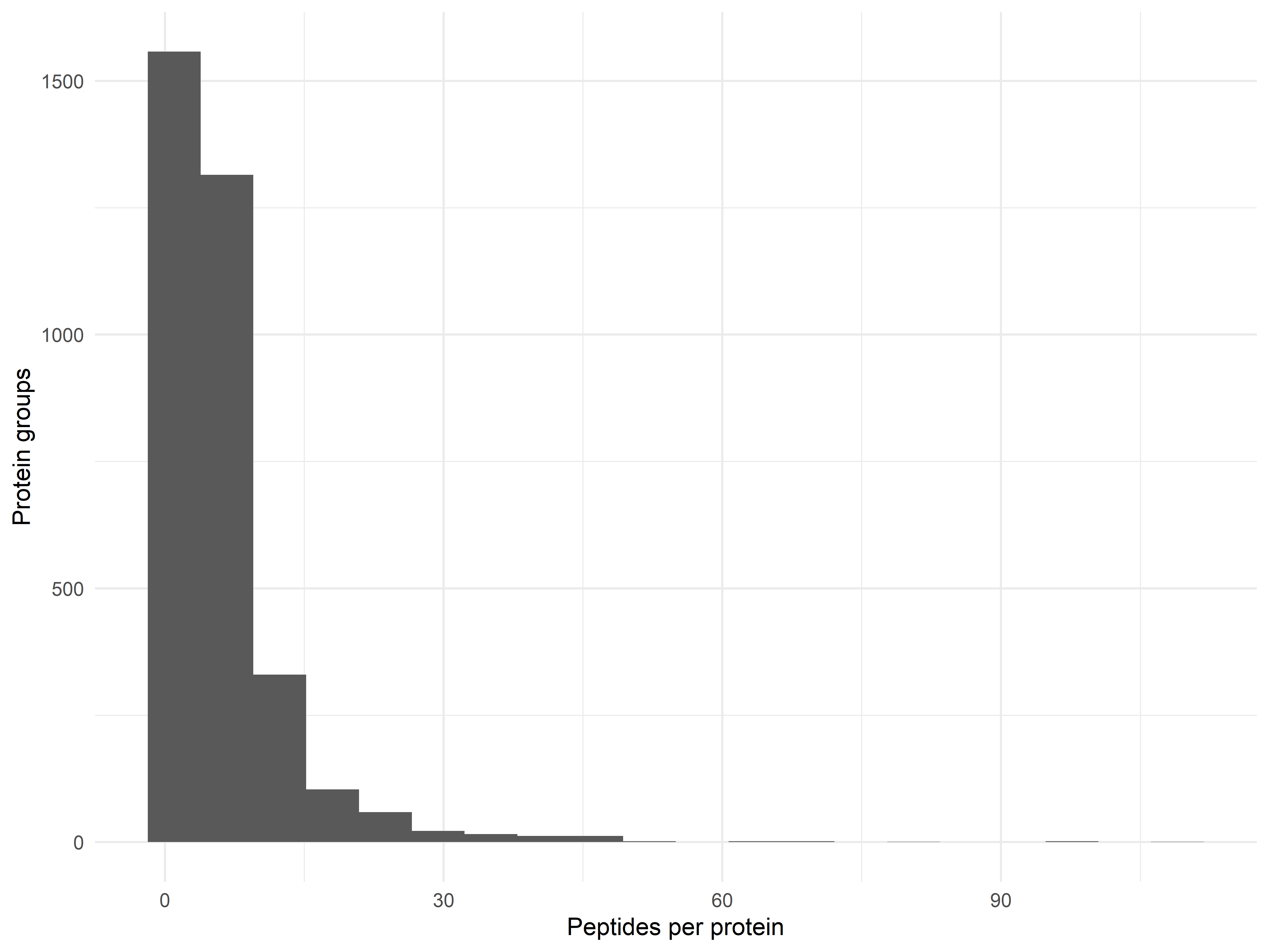
Aggregation collapses multiple quantitative observations (PSMs mapping to the same peptide, or peptides mapping to the same protein) into a single value per cell. The `scp` package uses `aggregateFeatures()` from `QFeatures`, which creates a new assay at each aggregation level.
The `leduc2022` dataset ships pre-aggregated, so we can inspect the peptide and protein assays directly rather than re-aggregating from the individual PSM files:
```{r}
#| eval: true
cat("Peptide assay dimensions:", dim(leduc[["peptides"]]), "\n")
cat("Protein assay dimensions:", dim(leduc[["proteins_processed"]]), "\n")
```
```
The `QFeatures` container retains all preceding assays, so you can always trace a protein's quantification back to its constituent peptides and PSMs:
```{r}
# Trace the provenance of a specific protein
which_protein <- "P14625" # example accession
provenance <- leduc |>
subsetByFeature(which_protein)
provenance
```
```{r}
#| eval: true
#| fig-cap: "Number of peptides per protein in the aggregated data."
peptides_per_protein <- rowData(leduc[["peptides"]]) |>
    as.data.frame() |>
    count(Leading.razor.protein)

qplot(peptides_per_protein$n, bins = 20) +
    labs(x = "Peptides per protein", y = "Protein groups") +
    theme_minimal()
```
## Normalization and Batch Assessment
### Normalization Strategy
SCP normalization must address technical variation between cells within a run and, when multiple runs are present, between runs. The `scp` package provides `normalizeScp()` for this purpose.
The key assumptions underlying median-based normalization in SCP are:
1. **Most proteins do not change** between the cells being compared — the median protein intensity is assumed stable.
2. **Technical variation is multiplicative** — a scaling factor per channel is sufficient to align the intensity distributions.
3. **The reference channel (if present) is compositionally identical across runs** — it serves as an anchor for cross-run scaling.
When these assumptions are violated — for example, when comparing very different cell types — more conservative normalization (e.g., quantile) or the use of spike-in controls may be warranted.
```{r}
#| eval: true
# Median normalization of the protein assay
prot_mat <- assay(leduc[["proteins_processed"]])
scale_factors <- apply(prot_mat, 2, median, na.rm = TRUE)
prot_norm <- sweep(prot_mat, 2, scale_factors, "/", check.margin = FALSE)

cat("Normalized protein matrix dimensions:", dim(prot_norm), "\n")
```
```{r}
#| eval: true
#| fig-cap: "Per-channel median intensity before and after normalization."
# Extract protein data before and after normalization
before <- assay(leduc[["proteins_processed"]])
after <- prot_norm

compare <- data.frame(
    channel = colnames(before),
    median_before = apply(before, 2, median, na.rm = TRUE),
    median_after = apply(after, 2, median, na.rm = TRUE)
) |>
    pivot_longer(-channel, names_to = "step", values_to = "median_intensity")

ggplot(compare, aes(x = step, y = log10(median_intensity), group = channel)) +
    geom_line(alpha = 0.5) +
    geom_point(aes(color = step)) +
    labs(x = "", y = "log10(median intensity)") +
    theme_minimal()
```
### Batch Assessment
In the `leduc2022` dataset, all cells come from a single TMTpro-16 run, so there is only one batch. The concepts below apply when your experiment includes multiple TMT runs.
```{r}
#| eval: true
#| fig-cap: "PCA of protein-level data colored by cell condition."
# Log-transform normalized protein data
prots_log <- log2(prot_norm + 1)

# Replace non-finite values with NA and keep proteins
# detected in at least 50 % of cells
prots_log[!is.finite(prots_log)] <- NA
detect_rate <- rowMeans(!is.na(prots_log))
prots_log <- prots_log[detect_rate >= 0.5, ]

# Impute remaining NAs with row means for PCA (prcomp cannot handle NAs)
k <- which(is.na(prots_log), arr.ind = TRUE)
if (nrow(k) > 0) {
    row_means <- rowMeans(prots_log, na.rm = TRUE)
    prots_log[k] <- row_means[k[, 1]]
}

# PCA
pca <- prcomp(t(prots_log), scale. = TRUE, center = TRUE)

# Prepare plot data using colData matching the assay columns
pca_data <- as.data.frame(pca$x)
pca_data$SampleType <- colData(leduc[["proteins_processed"]])$SampleType

pca_var <- summary(pca)$importance[2, 1:2] * 100  # variance explained

ggplot(pca_data, aes(x = PC1, y = PC2, color = SampleType)) +
    geom_point(size = 3) +
    stat_ellipse(level = 0.7, show.legend = FALSE) +
    labs(x = sprintf("PC1 (%.1f%%)", pca_var[1]),
         y = sprintf("PC2 (%.1f%%)", pca_var[2])) +
    scale_color_brewer(palette = "Set1") +
    theme_minimal()
```
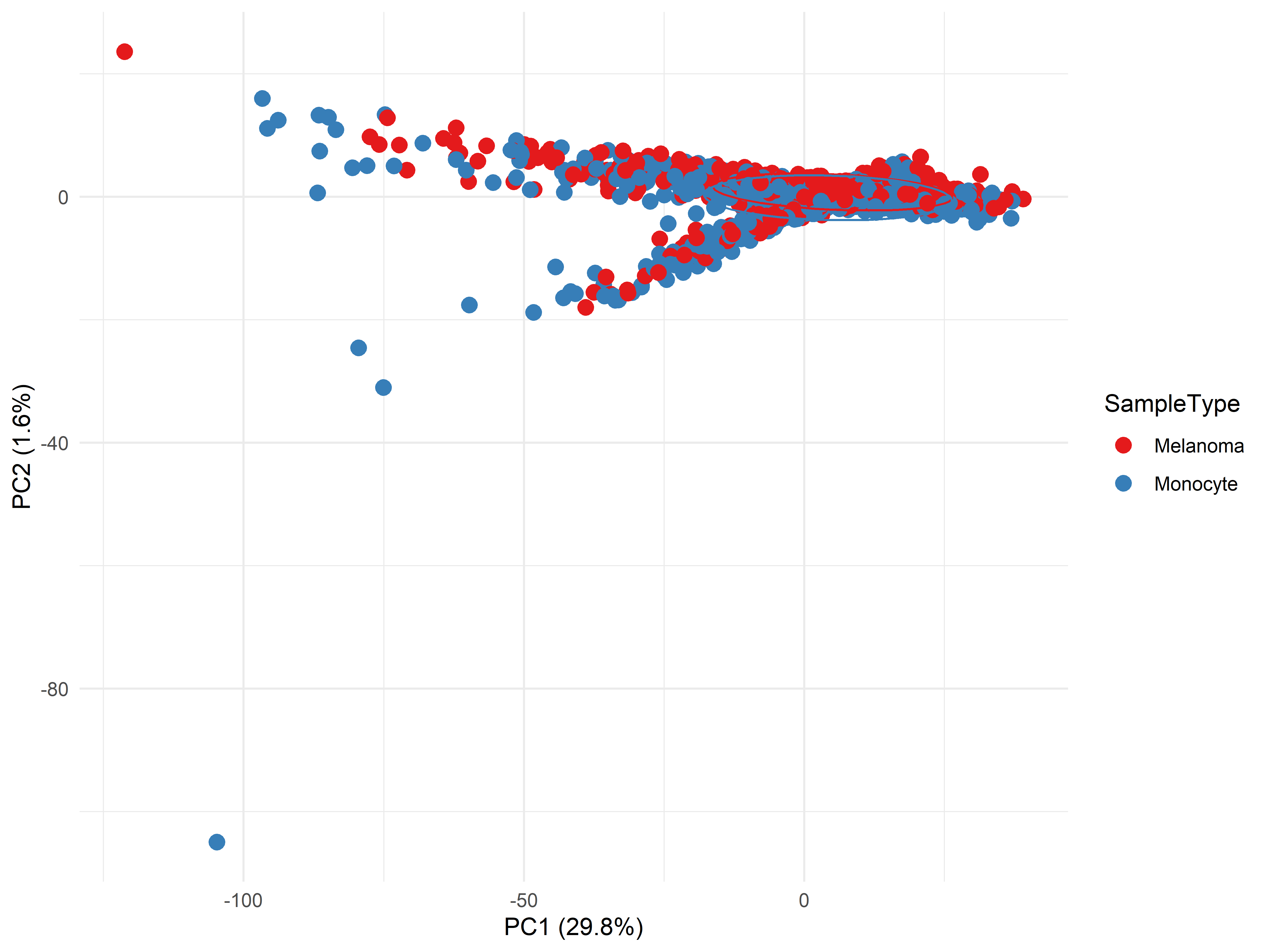
PCA separation by cell condition after normalization suggests that biological differences are recoverable despite technical variation. If PCA instead separated by acquisition run (in a multi-run experiment), that would signal a residual batch effect requiring additional correction. Approaches include using the reference channel for batch normalization or including batch as a covariate in the statistical model (see Chapter 18 for batch-effect concepts and Chapter 20 for mixed-effect modeling).
## Dimensional Reduction and Visualization
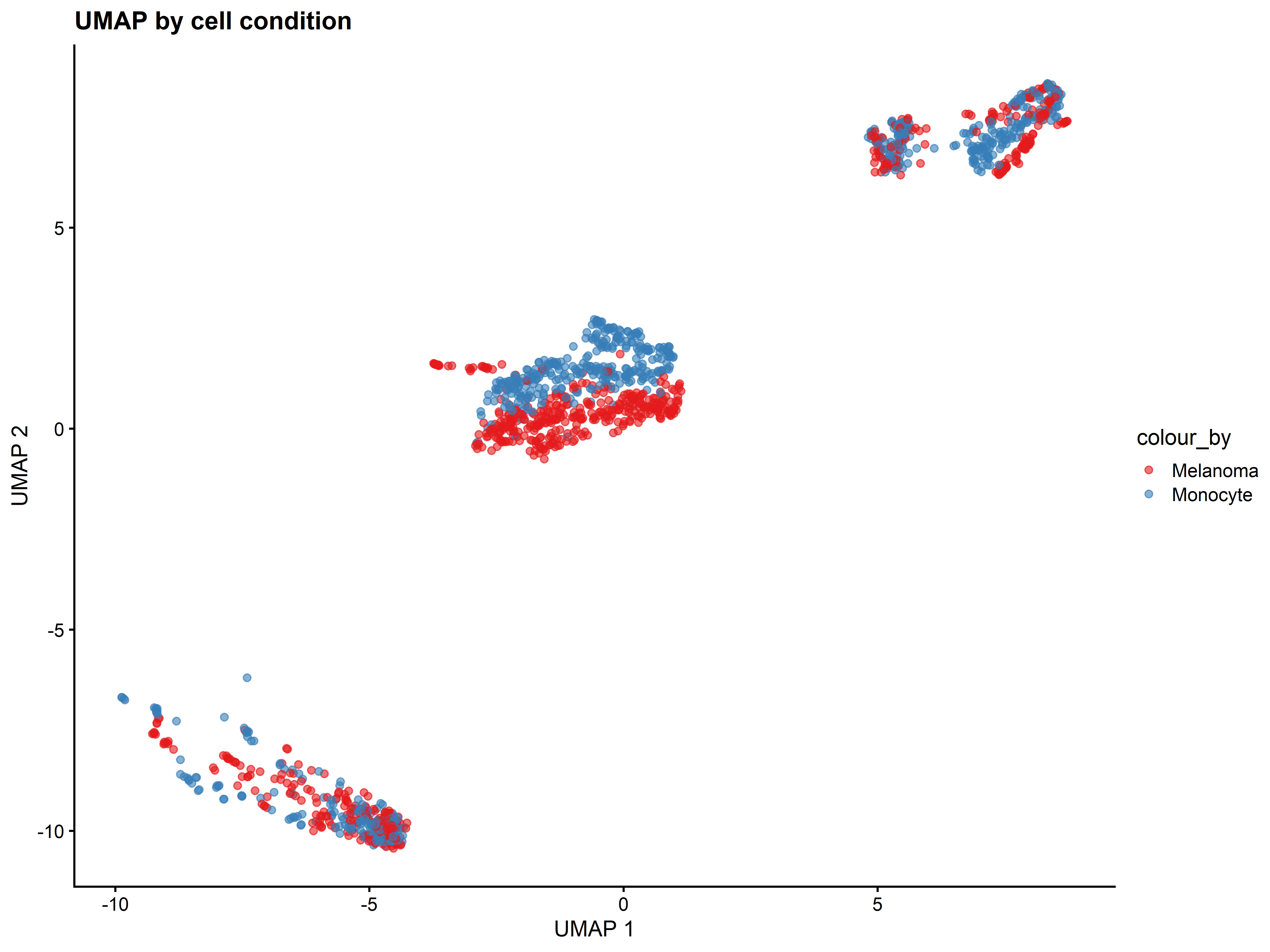
Beyond PCA, the `scater` package provides dedicated single-cell visualization methods. These help answer specific questions about data structure:
- **Do cells cluster by condition or by technical factors (run, channel position)?**
- **Are there outlier cells with unusual protein profiles?**
- **How much of the variance is explained by known biological and technical covariates?**
```{r}
#| eval: true
#| fig-cap: "UMAP embedding of single-cell proteome profiles, colored by cell condition."
# Create a SingleCellExperiment for scater functions
sce <- SingleCellExperiment(
    assays = list(logcounts = prots_log),
    colData = colData(leduc[["proteins_processed"]])
)

# Run UMAP (via scater which uses scater::runUMAP, itself wrapping uwot)
set.seed(2024)
sce <- runUMAP(sce)

plotUMAP(sce, colour_by = "SampleType") +
    scale_color_brewer(palette = "Set1") +
    labs(title = "UMAP by cell condition")
```
```{r}
#| eval: true
#| fig-cap: "Variance decomposition of protein expression across known covariates."
# Variance explained by condition vs other available covariates
# This uses variancePartition-style logic as shown in Chapter 20
if (requireNamespace("variancePartition", quietly = TRUE)) {
    tryCatch({
        library(variancePartition)
        # Build formula with available covariates from colData
        form <- ~ SampleType + Channel
        varPart <- fitExtractVarPartModel(prots_log, form, colData(leduc[["proteins_processed"]]))
        plotVarPart(sortCols(varPart)) +
            labs(title = "Variance decomposition")
    }, error = function(e) {
        cat("Variance decomposition skipped (package compatibility issue):\n  ", conditionMessage(e), "\n")
    })
} else {
    cat("Install variancePartition for variance decomposition analysis.\n")
}
```
::: {.callout-tip title="When to use scater vs. scp functions"}
Use `scp::scp_qc()` and `scp::normalizeScp()` for SCP-specific operations (QC metrics, normalization within the QFeatures hierarchy). Use `scater::plotPCA()`, `scater::runUMAP()`, and `scater::plotColData()` for exploratory visualization that benefits from single-cell-oriented defaults (point transparency, color scales, feature-name annotation).
:::
## Statistical Modeling
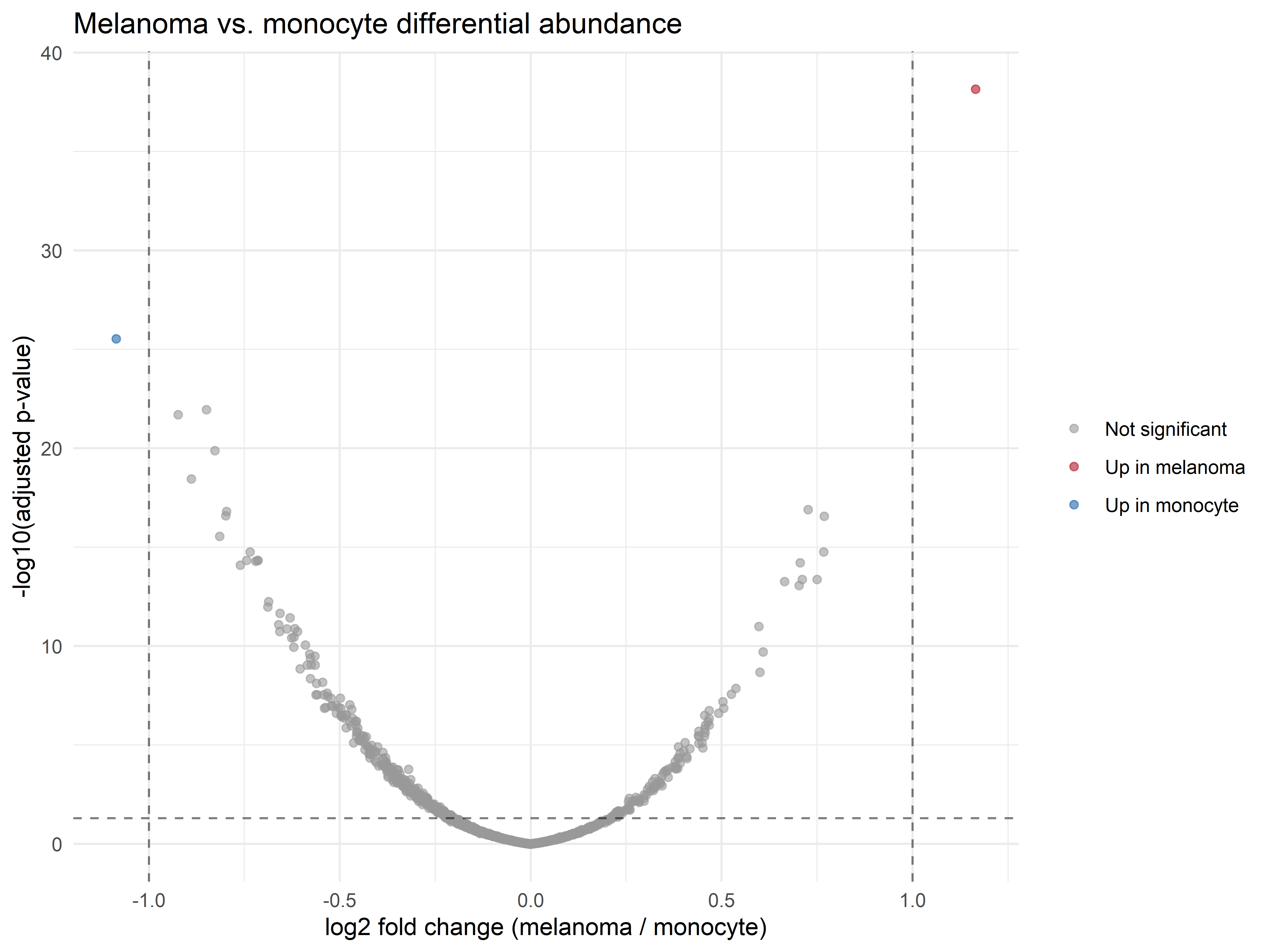
Differential abundance analysis in SCP faces two challenges: the high proportion of missing values and the modest number of cells per condition (often 10–50). The principles from the book's statistical chapters apply with the following adjustments:
- **Design matrices** follow the same structure as Chapter 19 (two-group, multi-group, or factorial designs). For the `leduc2022` dataset, compare naive vs. primed conditions.
- **Empirical Bayes moderation** (`limma`, Chapter 19) can be applied to the protein-level matrix after filtering out proteins with excessive missingness. Limma's moderated *t*-test stabilizes variance estimates when the number of cells is small.
- **Missing values** must be handled before limma. A common SCP strategy is to keep only proteins detected in at least 50–70 % of cells in at least one condition, then impute the remaining missing values per condition (e.g., with `impute::impute.knn()` or minimum-value imputation). Be aware that the choice of imputation method can strongly affect the results; see Chapter 18 for imputation sensitivity analysis.
- **Mixed models** (Chapter 20) are appropriate when multiple acquisition runs exist, with `SampleType` as a fixed effect and `Run` as a random intercept: `~ SampleType + (1 | Run)`.
```{r}
#| eval: true
#| fig-cap: "Volcano plot comparing melanoma vs. monocyte cells."
# Filter: keep proteins with at least 50% detection in at least one condition
keep <- apply(prots_log, 1, function(x) {
    by_cond <- split(x, colData(leduc[["proteins_processed"]])$SampleType)
    any(sapply(by_cond, function(y) mean(!is.na(y)) >= 0.5))
})
prots_filt <- prots_log[keep, ]
cat("Proteins retained after filtering:", sum(keep), "/", nrow(prots_log), "\n")
# Simple imputation by condition median
prots_imp <- prots_filt
for (cond in unique(colData(leduc[["proteins_processed"]])$SampleType)) {
    idx <- colData(leduc[["proteins_processed"]])$SampleType == cond
    for (i in seq_len(nrow(prots_imp))) {
        if (is.na(prots_imp[i, idx][1])) {
            cond_vals <- prots_filt[i, idx]
            prots_imp[i, idx][is.na(prots_imp[i, idx])] <-
                median(cond_vals, na.rm = TRUE)
        }
    }
}

# limma differential abundance (Melanoma vs Monocyte)
library(limma)
cd <- colData(leduc[["proteins_processed"]])
design <- model.matrix(~ 0 + cd$SampleType)
colnames(design) <- levels(factor(cd$SampleType))
fit <- lmFit(prots_imp, design)
cont <- makeContrasts(
    melanoma_vs_monocyte = Melanoma - Monocyte,
    levels = design
)
fit2 <- contrasts.fit(fit, cont)
fit2 <- eBayes(fit2)
tt <- topTable(fit2, number = Inf)

# Volcano plot
tt$sig <- ifelse(tt$adj.P.Val < 0.05 & abs(tt$logFC) > 1,
    ifelse(tt$logFC > 0, "Up in melanoma", "Up in monocyte"),
    "Not significant"
)

ggplot(tt, aes(x = logFC, y = -log10(adj.P.Val), color = sig)) +
    geom_point(alpha = 0.6) +
    geom_hline(yintercept = -log10(0.05), linetype = "dashed", alpha = 0.5) +
    geom_vline(xintercept = c(-1, 1), linetype = "dashed", alpha = 0.5) +
    scale_color_manual(values = c("Up in monocyte" = "#2166AC",
                                   "Not significant" = "grey60",
                                   "Up in melanoma" = "#B2182B")) +
    labs(x = "log2 fold change (melanoma / monocyte)",
         y = "-log10(adjusted p-value)",
         title = "Melanoma vs. monocyte differential abundance") +
    theme_minimal() +
    theme(legend.title = element_blank())
```
```{r}
#| eval: true
cat("Top differentially abundant proteins (melanoma vs. monocyte):\n")
tt |>
    filter(adj.P.Val < 0.05) |>
    arrange(adj.P.Val) |>
    head(10)
```
::: {.callout-warning title="Biological replication matters"}
The differential analysis above uses cells as observations. These are **technical replicates** of the cell-culture condition, not independent biological replicates. A finding that holds across cells from one culture may not generalize to cells from an independently cultured population. For publication-level results, plan experiments with multiple biological replicates (independent cultures or tissue samples), with each replicate contributing several cells to a TMT run.
:::
## Summary
Single-cell proteomics analysis with `scp` adapts the familiar `QFeatures` framework to the unique challenges of low-input proteomics:
- **Data model**: `scp` stores acquisition runs as `SingleCellExperiment` assays within a `QFeatures` container, providing access to both `QFeatures` aggregation methods and `scater`/`scran` single-cell visualisation and normalization functions.
- **QC**: The `scp_qc()` function computes per-channel identification counts, total intensity, and missingness proportions, flagging problematic channels (doublets, empty channels, failed labeling).
- **Filtering and aggregation**: Standard PSM-level filters (remove reverse hits, contaminants, low PEP score) precede aggregation PSM → peptide → protein via `aggregateFeatures()`.
- **Normalization**: Median-based scaling per channel, anchored by a reference channel when available, aligns intensity distributions across cells within and between runs.
- **Visualization**: PCA and UMAP (via `scater`) reveal structure driven by cell condition, run, or channel position.
- **Statistical modeling**: The limma framework from Chapter 19 applies after filtering and imputation, with the caveat that cell-level replication does not substitute for biological replication.
## Exercises
1. **Subsetting practice.** Filter the `leduc` object to keep only the naive and primed conditions, then repeat the PCA. Does the separation improve?
2. **Normalization comparison.** Replace the median normalization with `method = "colScale"` in `normalizeScp()`. Compare the PCA before and after this alternative normalization.
3. **Missingness filtering.** Vary the detection-rate threshold (used in the statistical modeling section) from 30 % to 70 %. How does the number of retained proteins and the number of significant hits change?
4. **Multi-run workflow (conceptual).** If your experiment had three TMTpro-16 runs, which steps would change? Describe how `joinAssays()` fits into the pipeline and where the reference channel is used for batch normalization.
5. **Cross-reference with Chapter 20.** The limma analysis in this appendix compares two groups (naive vs. primed). If the experiment added a third condition (e.g., reset), what design matrix and contrasts would you use? Write the `model.matrix()` call.
## Session Information
```{r}
#| eval: true
sessionInfo()
```