# Targeted MS Quantification and Calibration
> *In targeted metabolomics, the question is not only whether a molecule is present, but how much is there and how confident you are.*
Targeted mass spectrometry (MS) quantifies pre-selected metabolites with high sensitivity, specificity, and linear dynamic range. This chapter covers the principles of targeted quantification – from assay design to absolute concentration determination – and provides a practical R workflow for building calibration curves, calculating limits, and reporting results.
---
::: {.callout-warning title="The One Mistake to Avoid"}
Reporting concentrations outside the calibration range. A value above your highest standard or below the LOQ is a guess dressed as a measurement. Report only within the validated linear range.
:::
## Learning Objectives
By the end of this chapter, you will be able to:
- Distinguish targeted (**SRM/MRM/PRM**) from untargeted MS workflows
- Construct and evaluate a **calibration curve** for a metabolite
- Use **internal standards** to correct for matrix effects and instrument drift
- Compute **limit of detection (LOD)** and **limit of quantification (LOQ)**
- Perform **peak integration** and manual QC
- Implement a complete targeted quantification pipeline in R
---
## Targeted Versus Untargeted Metabolomics
| Feature | Untargeted | Targeted |
|---------|-----------|----------|
| **Goal** | Discovery of unknown/known features | Precise quantification of known metabolites |
| **Coverage** | Hundreds to thousands | Tens to hundreds (pre-selected) |
| **Data type** | Full scan MS1 + data-dependent MS2 | Selected reaction monitoring (SRM/MRM) or parallel reaction monitoring (PRM) |
| **Sensitivity** | Moderate (µM range) | High (nM to pM range) |
| **Dynamic range** | 2–3 orders of magnitude | 4–6 orders of magnitude |
| **Quantification** | Semi-quantitative (relative) | Absolute (with standards) |
| **Throughput** | Low to medium | High (triple quadrupoles) |
**When to use targeted:** Hypothesis-driven studies, clinical biomarker validation, pathway analysis where absolute concentrations matter, or when measuring low-abundance metabolites in complex matrices.
---
## SRM, MRM, and PRM Data
### Basic Concepts
- **SRM (Selected Reaction Monitoring):** Single precursor ion → single product ion. Used on triple quadrupoles.
- **MRM (Multiple Reaction Monitoring):** Monitor multiple SRM transitions in one run (the common term).
- **PRM (Parallel Reaction Monitoring):** High-resolution MS2 (Q-Orbitrap) – all product ions from a precursor are monitored simultaneously.
### Transition Selection
For each metabolite, you need:
- **Precursor m/z** (usually [M+H]⁺ or [M-H]⁻)
- **Product ion m/z** (most intense, specific fragment)
- **Collision energy** (optimised for the transition)
Example: **Glucose** (negative mode)
Precursor: \( m/z \) 179.056 ([M-H]⁻) → Product: \( m/z \) 89.024 (fragment)
### Data Structure
Targeted data is usually a table with columns:
- `transition_id` (e.g., "glucose_179>89")
- `sample_id`
- `peak_area` (integrated intensity)
- `retention_time`
- `peak_width`, `signal_to_noise`, etc.
---
## Calibration Curves
### Principle
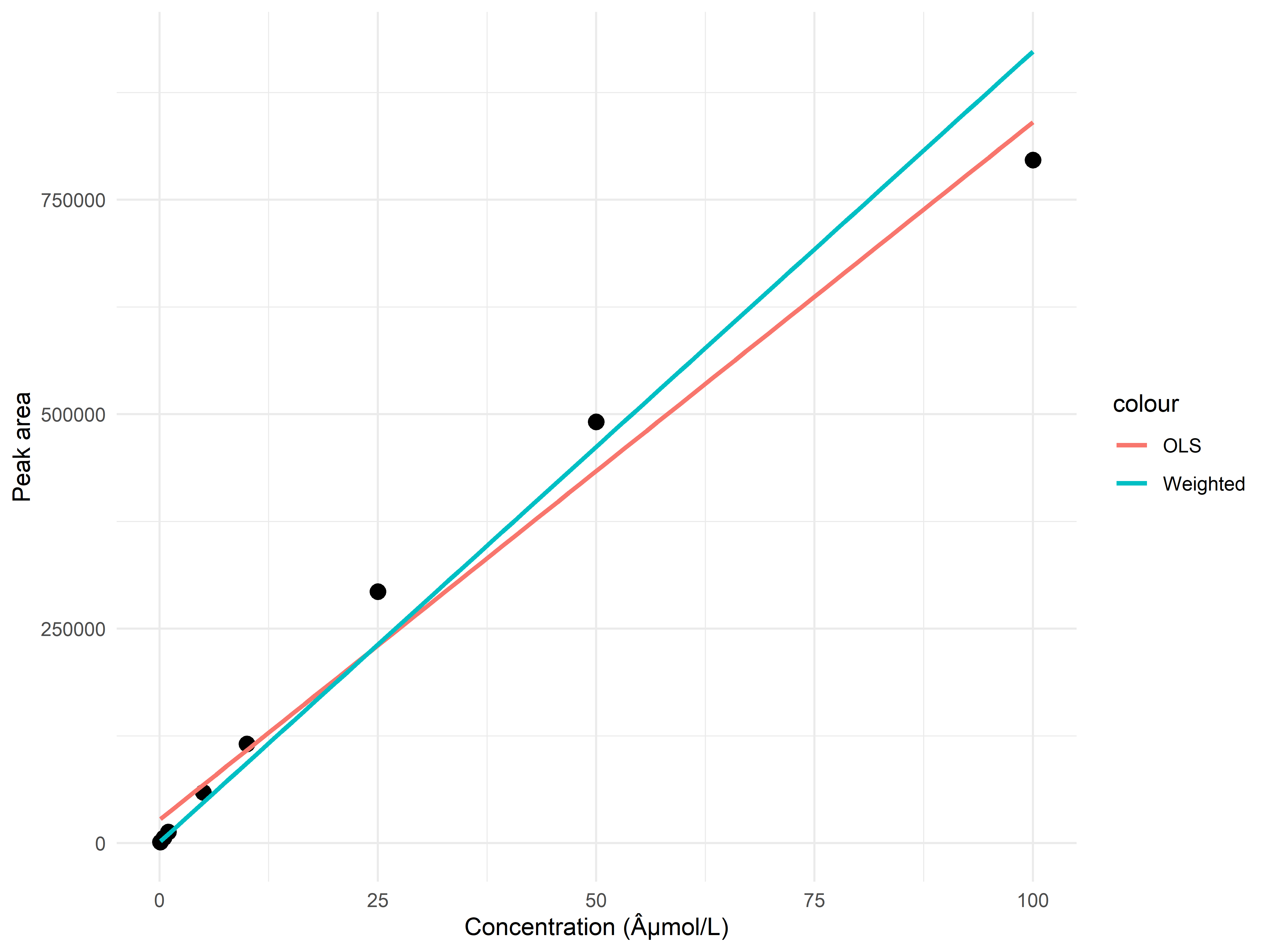
A calibration curve relates **known concentrations** of authentic standards to **measured peak areas** (or area ratios). It allows quantification of unknown samples by interpolation.
### Types of Calibration Models
| Model | Equation | When to use |
|-------|----------|--------------|
| Linear (unweighted) | \( A = a \cdot C + b \) | Low concentration range, constant variance |
| Linear (weighted) | \( A = a \cdot C + b \) with \( 1/x \) or \( 1/x^2 \) weights | Heteroscedastic data (common in MS) |
| Quadratic | \( A = a \cdot C^2 + b \cdot C + c \) | When linearity fails at high end |
### Building a Calibration Curve in R
```{r}
# Example data: glucose standard curve
calib_data <- data.frame(
  conc_umol_L = c(0.1, 0.5, 1, 5, 10, 25, 50, 100),
  area = c(1250, 6200, 12100, 59000, 115000, 270000, 480000, 850000)
)

# Add error (5% CV for simulation)
set.seed(123)
calib_data$area <- calib_data$area * (1 + rnorm(nrow(calib_data), 0, 0.05))

# Linear model (ordinary least squares)
lm_fit <- lm(area ~ conc_umol_L, data = calib_data)
summary(lm_fit)
# Weighted linear model (1/x weighting)
# Weight = 1 / (predicted variance) ~ 1/conc
lm_weighted <- lm(area ~ conc_umol_L, data = calib_data, weights = 1/conc_umol_L)

# Compare fits
library(ggplot2)
ggplot(calib_data, aes(x = conc_umol_L, y = area)) +
  geom_point(size = 3) +
  geom_smooth(method = "lm", se = FALSE, aes(color = "OLS")) +
  geom_smooth(method = "lm", se = FALSE, aes(weight = 1/conc_umol_L, color = "Weighted")) +
  labs(x = "Concentration (µmol/L)", y = "Peak area") +
  theme_minimal()
```
### Important Metrics
- **R²:** Goodness of fit (>0.99 for quantification)
- **Residuals:** Should be random and homoscedastic (check plot)
- **Back-calculated concentrations:** Should be within ±20% (or ±15% for bioanalysis)
```{r}
# Back-calculate standards
calib_data$conc_back <- (calib_data$area - coef(lm_fit)[1]) / coef(lm_fit)[2]
calib_data$accuracy <- (calib_data$conc_back / calib_data$conc_umol_L) * 100
print(calib_data[, c("conc_umol_L", "conc_back", "accuracy")])
```
---
## Internal Standards (IS)
### Why Use Internal Standards?
- Compensate for **matrix effects** (ion suppression/enhancement)
- Correct for **sample preparation losses** (extraction, derivatisation)
- Adjust for **instrument drift** (over long batches)
### Properties of a Good Internal Standard
| Property | Ideal |
|----------|-------|
| Chemical similarity | Same class, similar structure |
| Not naturally present | Stable isotope labelled (SIL) or unnatural analogue |
| Same extraction and LC behaviour | Closely matching retention time |
| Different mass | >3 Da from analyte (to avoid cross-talk) |
**Stable isotope labelled (SIL) standards** are gold standard: e.g., glucose-¹³C₆, tryptophan-d₅.
### Using IS in Calibration
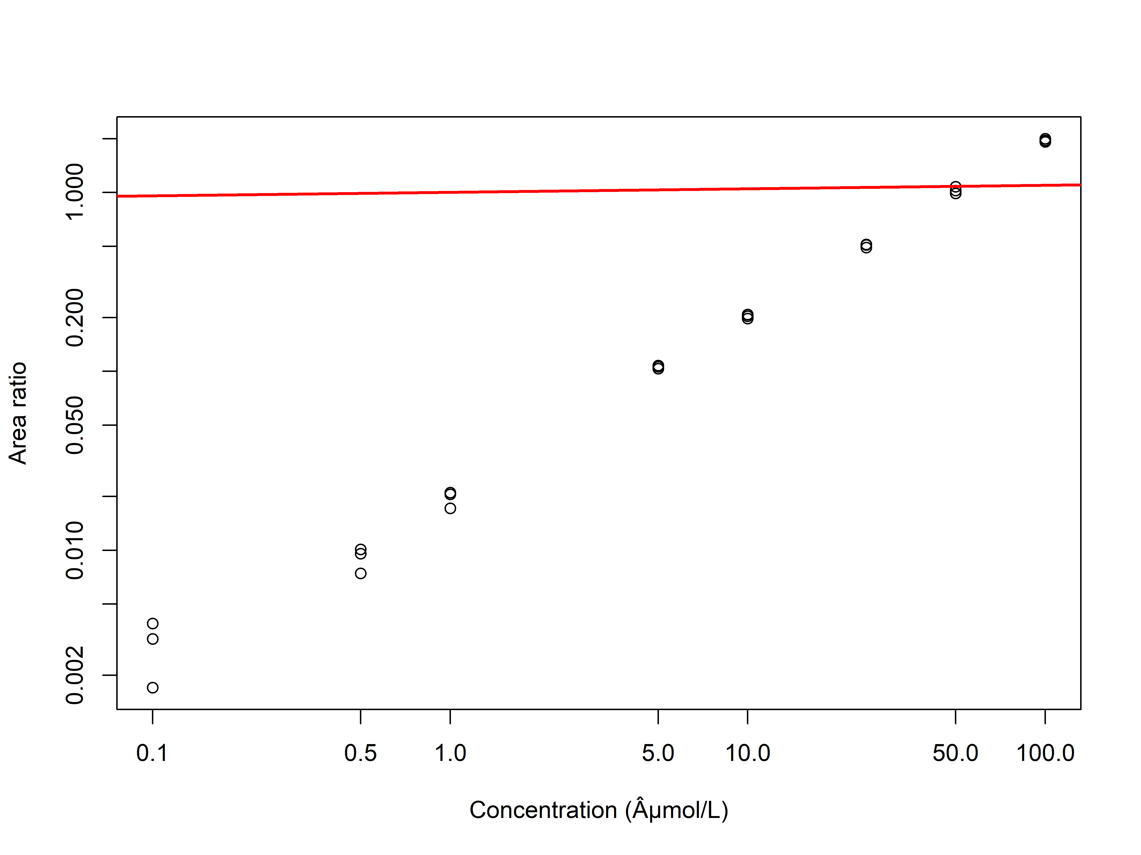
Instead of plotting **area** vs concentration, plot **area ratio** (analyte area / IS area) vs concentration. This normalises for IS recovery.
```{r}
# Example with IS
calib_is <- data.frame(
  conc = c(0.1, 0.5, 1, 5, 10, 25, 50, 100),
  area_ratio = c(0.012, 0.060, 0.118, 0.585, 1.125, 2.68, 5.10, 9.20)
)

lm_ratio <- lm(area_ratio ~ conc, data = calib_is)
summary(lm_ratio)  # Should have near-zero intercept if IS works well
```
**Check for IS consistency:** IS peak area should be constant across all samples (CV < 20%). Large variation indicates injection or extraction problems.
---
## Limit of Detection and Limit of Quantification
### Definitions
- **LOD** – lowest concentration that can be reliably detected (signal > noise, typically S/N ≥ 3)
- **LOQ** – lowest concentration that can be quantified with acceptable precision and accuracy (S/N ≥ 10, CV < 20%)
### Empirical Calculation from Calibration Data
**Method 1 – Using blank replicates:**
```{r}
# Measure 10 blanks, compute mean and SD of peak area
blanks <- c(125, 98, 145, 110, 135, 118, 140, 122, 108, 130)
blank_mean <- mean(blanks)
blank_sd <- sd(blanks)

lod_area <- blank_mean + 3 * blank_sd
loq_area <- blank_mean + 10 * blank_sd

# Convert to concentration using calibration curve
# Assumes calibration near zero is linear
slope <- coef(lm_fit)[2]
lod_conc <- (lod_area - coef(lm_fit)[1]) / slope
loq_conc <- (loq_area - coef(lm_fit)[1]) / slope

cat("LOD =", lod_conc, "µmol/L\n")
cat("LOQ =", loq_conc, "µmol/L\n")
```
**Method 2 – Signal-to-noise ratio:**
If your software reports S/N, you can compute:
```{r}
# For a low concentration standard that gives S/N ~ 3
# LOD = conc_std * (3 / S_N_std)
s_n_std <- 12   # measured S/N at 0.5 µmol/L
conc_std <- 0.5
lod <- conc_std * (3 / s_n_std)    # 0.125 µmol/L
```
### Reporting Rules
- Concentrations < LOD → report as `< LOD` (or `0`)
- LOD ≤ concentration < LOQ → report with note: “estimated, below LOQ”
- Concentration ≥ LOQ → report numerical value
---
## Peak Integration and Manual Inspection
### Automated Integration
Most software (Xcalibur, Analyst, Skyline) integrates peaks automatically using algorithms:
- **Gaussian fit** – assumes symmetrical peak shape
- **Centroid** – uses apex only (less accurate for quantification)
- **Sum of raw intensities** – over a manually defined time window
### Common Integration Errors
| Error | Example | Fix |
|-------|---------|-----|
| Baseline drift | Rising baseline under peak | Manual baseline adjustment |
| Shoulder / split peak | Co-eluting isomer | Adjust integration boundaries or use deconvolution |
| Noise as peak | Small spike near LOD | Set S/N threshold or review manually |
| Wrong peak assignment | Wrong transition or retention time shift | Re-align RT (dynamic RT window) |
### Manual Validation Workflow
For **targeted quantification**, always review each integration visually. Use a script that flags suspicious peaks:
```{r}
library(dplyr)
# Simulated peak data
peak_data <- data.frame(
  transition = "glucose_179>89",
  sample = c("Std_1", "Std_2", "Unknown_1", "QC_1"),
  area = c(12000, 11800, 999999, 11500),   # outlier in unknown
  rt = c(2.35, 2.36, 2.37, 2.34),
  sn_ratio = c(35, 33, 5, 31)               # low S/N for unknown
)

# Flag problematic peaks
peak_data <- peak_data %>%
  mutate(
    flag = case_when(
      area > 5 * median(area) ~ "Outlier area",
      sn_ratio < 10 ~ "Low S/N (<10)",
      rt < 2.3 | rt > 2.4 ~ "RT shift",
      TRUE ~ "OK"
    )
  )
filter(peak_data, flag != "OK")
```
**Best practice:** For publication-quality data, manually inspect **all flagged peaks** and at least 10% of random peaks.
---
## Absolute Versus Relative Quantification
| | Absolute Quantification | Relative Quantification |
|---|------------------------|-------------------------|
| **Requires** | Authentic calibration curve, internal standard | None (or pooled QC) |
| **Output** | Concentration (e.g., 15.3 nmol/L) | Fold change, ratio |
| **Used for** | Biomarker cut-offs, flux analysis, excretion studies | Discovery, comparing treatments |
| **Inter-batch** | Can compare across batches (with IS) | Requires batch correction (e.g., QC normalisation) |
### Semi-Quantitative Workflow (No Standards)
Use **pooled quality control (QC)** samples injected throughout the run:
```{r}
#| eval: false
# Relative quantification: divide each sample by median of QCs for that feature
# Assume long_format data: sample_id, metabolite, area
rel_quant <- long_data %>%
  group_by(metabolite) %>%
  mutate(
    qc_median = median(area[sample_type == "QC"], na.rm = TRUE),
    relative_area = area / qc_median
  ) %>%
  ungroup()
```
---
## Practical Example: Targeted Metabolite Quantification in R
We will run a complete targeted quantification pipeline using simulated data:
1. **Read calibration standards and internal standard data**
2. **Build calibration curve with weighting**
3. **Calculate LOD/LOQ**
4. **Apply to unknown samples**
5. **Report final concentrations**
### Step 1 – Load and explore data
```{r}
# Simulate dataset
set.seed(42)

# Standards (5 concentration levels, triplicates)
calib <- expand.grid(
  conc_umol = c(0.1, 0.5, 1.0, 5.0, 10.0, 25.0, 50.0, 100.0),
  rep = 1:3
)
calib$area_analyte <- with(calib, 10000 * conc_umol + rnorm(nrow(calib), 0, 500))
calib$area_IS <- 500000 + rnorm(nrow(calib), 0, 15000)
calib$area_ratio <- calib$area_analyte / calib$area_IS

# Unknown samples (n = 20)
unknowns <- data.frame(
  sample_id = paste0("S", 1:20),
  area_analyte = runif(20, 5000, 800000),
  area_IS = 500000 + rnorm(20, 0, 20000)
)
unknowns$area_ratio <- unknowns$area_analyte / unknowns$area_IS
```
### Step 2 – Build calibration curve
```{r}
# Weighted linear regression (1/x^2)
weights <- 1 / (calib$conc_umol^2)
calib_model <- lm(area_ratio ~ conc_umol, data = calib, weights = weights)

summary(calib_model)
# Plot
plot(calib$conc_umol, calib$area_ratio, log = "xy",
     xlab = "Concentration (µmol/L)", ylab = "Area ratio")
abline(calib_model, col = "red", lwd = 2)
```
### Step 3 – Determine LOD and LOQ using blank
```{r}
# Simulate 10 blanks
blanks <- data.frame(area_ratio = rnorm(10, 0.001, 0.0003))
blank_sd <- sd(blanks$area_ratio)
lod_ratio <- mean(blanks$area_ratio) + 3 * blank_sd
loq_ratio <- mean(blanks$area_ratio) + 10 * blank_sd

# Convert to concentration (using the calibration model)
lod_conc <- (lod_ratio - coef(calib_model)[1]) / coef(calib_model)[2]
loq_conc <- (loq_ratio - coef(calib_model)[1]) / coef(calib_model)[2]

cat("LOD =", round(lod_conc, 3), "µmol/L\n")
cat("LOQ =", round(loq_conc, 3), "µmol/L\n")
```
### Step 4 – Quantify unknowns and flag below LOD/LOQ
```{r}
unknowns$conc_umol <- (unknowns$area_ratio - coef(calib_model)[1]) / coef(calib_model)[2]
unknowns$quant_status <- case_when(
  unknowns$conc_umol < lod_conc ~ "< LOD",
  unknowns$conc_umol < loq_conc ~ "< LOQ",
  TRUE ~ "OK"
)

# Replace values below LOD with NA or 0
unknowns$conc_umol_final <- ifelse(unknowns$conc_umol < loq_conc, NA, unknowns$conc_umol)

head(unknowns)
```
### Step 5 – Quality control and reporting
```{r}
# CV of IS across all samples
IS_cv <- sd(unknowns$area_IS) / mean(unknowns$area_IS) * 100
cat("IS CV =", round(IS_cv, 1), "%")
# Summary table of quantified concentrations
summary_table <- unknowns %>%
  group_by(quant_status) %>%
  summarise(n = n(), mean_conc = mean(conc_umol_final, na.rm = TRUE))

print(summary_table)
# Export results
write.csv(unknowns, "targeted_quant_results.csv", row.names = FALSE)
```
---
## Example 4: Targeted MS Calibration and Quantitative Assay Report
### Project Question
Can we quantify predefined peptides or metabolites reliably using targeted MS?
This example teaches assay-style reporting. The goal is not discovery but defensible quantification of predefined analytes, supported by transition-level evidence, calibration performance, precision, LOD, LOQ, and clear result flags.
### Dataset and Scope
Use an MSstats-compatible targeted table, a Skyline/Panorama export, Panorama Public subset, or the simulated calibration dataset below. `MSstats` supports statistical relative quantification for targeted data (see Chapter 12 for the full MSstats ecosystem overview); the calibration components here are written in plain R so they can also be used for small-molecule targeted assays.
### Workflow Map
| Step | Implementation |
|---|---|
| Metadata and contrasts | Define calibrators, QC samples, unknown samples, conditions, analytes, and transitions |
| Import | Read a Skyline, Panorama, or MSstats-compatible transition-level table |
| Raw/run-level QC | Inspect transition peak areas, retention-time consistency, and replicate precision |
| Transition audit | Remove unreliable transitions with low S/N, RT drift, poor precision, or missing peaks |
| Abundance matrix | Summarize transitions to peptide, protein, or metabolite abundance |
| Low-quality filtering | Remove blank-contaminated analytes and high-CV QC analytes |
| Normalization | Apply internal-standard correction and log2 transformation when appropriate |
| Missingness diagnosis | Check failed injections and missing transitions |
| Statistical modeling | Fit calibration curves and, when needed, group comparison models |
| Multiple testing | Apply FDR if many analytes are tested |
| Visualization | Calibration curve, residual plot, precision plot, group comparison plot |
| Biological interpretation | Interpret targeted analytes in the intended pathway or assay context |
| Reproducible export | Save assay report with calibration, LOD/LOQ, precision, flags, and results |
### Simulate a Transition-Level Assay Table
```{r}
#| eval: false
library(dplyr)
library(tidyr)
library(purrr)
library(broom)
library(ggplot2)
library(gt)
library(sessioninfo)

set.seed(4)

dir.create("results", showWarnings = FALSE)
dir.create("figures", showWarnings = FALSE)
dir.create("objects", showWarnings = FALSE)

analytes <- tibble(
  analyte = c("Tryptophan", "Kynurenine", "Phenylalanine"),
  internal_standard = c("Tryptophan_d5", "Kynurenine_d4", "Phenylalanine_d5"),
  slope = c(0.018, 0.026, 0.014),
  intercept = c(0.001, 0.0015, 0.0008)
)

calibrators <- expand_grid(
  analyte = analytes$analyte,
  concentration_nM = c(0, 1, 5, 10, 25, 50, 100, 250, 500),
  replicate = 1:3,
  transition = c("quantifier", "qualifier")
) |>
  left_join(analytes, by = "analyte") |>
  mutate(
    sample_type = if_else(concentration_nM == 0, "blank", "calibrator"),
    sample_id = paste(sample_type, analyte, concentration_nM, replicate, sep = "_"),
    area_is = rlnorm(n(), log(5e5), 0.08),
    transition_factor = if_else(transition == "quantifier", 1, 0.55),
    area_ratio = pmax(intercept + slope * concentration_nM, 0) * transition_factor *
+      rlnorm(n(), 0, 0.08),
    area_analyte = area_ratio * area_is,
    retention_time = case_when(
      analyte == "Tryptophan" ~ 4.2,
      analyte == "Kynurenine" ~ 3.1,
      TRUE ~ 5.4
    ) + rnorm(n(), 0, 0.025),
    signal_to_noise = if_else(concentration_nM == 0, runif(n(), 1, 3), runif(n(), 20, 200))
  )

qc_unknowns <- expand_grid(
  analyte = analytes$analyte,
  sample_id = c(paste0("QC_", 1:6), paste0("Sample_", 1:18)),
  transition = c("quantifier", "qualifier")
) |>
  left_join(analytes, by = "analyte") |>
  mutate(
    sample_type = if_else(grepl("^QC", sample_id), "QC", "unknown"),
    condition = if_else(as.integer(gsub("Sample_", "", sample_id)) <= 9, "Control", "Treatment"),
    true_concentration_nM = case_when(
      sample_type == "QC" ~ 50,
      analyte == "Kynurenine" & condition == "Treatment" ~ 85,
      TRUE ~ runif(n(), 20, 80)
    ),
    area_is = rlnorm(n(), log(5e5), 0.10),
    transition_factor = if_else(transition == "quantifier", 1, 0.55),
    area_ratio = (intercept + slope * true_concentration_nM) * transition_factor *
+      rlnorm(n(), 0, 0.10),
    area_analyte = area_ratio * area_is,
    retention_time = case_when(
      analyte == "Tryptophan" ~ 4.2,
      analyte == "Kynurenine" ~ 3.1,
      TRUE ~ 5.4
    ) + rnorm(n(), 0, 0.035),
    signal_to_noise = runif(n(), 15, 150),
    concentration_nM = NA_real_,
    replicate = NA_integer_
  )

targeted_long <- bind_rows(calibrators, qc_unknowns) |>
  select(sample_id, sample_type, condition, analyte, transition,
         concentration_nM, replicate, area_analyte, area_is, area_ratio,
         retention_time, signal_to_noise)

write_csv(targeted_long, "results/targeted_01_transition_level_table.csv")
```
### Transition-Level QC
```{r}
#| eval: false
transition_qc <- targeted_long |>
  group_by(analyte, transition, sample_type) |>
  summarise(
    n = n(),
    pct_missing = mean(is.na(area_analyte) | area_analyte <= 0) * 100,
    median_rt = median(retention_time, na.rm = TRUE),
    rt_sd = sd(retention_time, na.rm = TRUE),
    median_sn = median(signal_to_noise, na.rm = TRUE),
    cv_area_ratio = sd(area_ratio, na.rm = TRUE) / mean(area_ratio, na.rm = TRUE) * 100,
    .groups = "drop"
  ) |>
  mutate(
    qc_flag = case_when(
      pct_missing > 20 ~ "high missingness",
      rt_sd > 0.10 ~ "RT instability",
      median_sn < 10 ~ "low signal-to-noise",
      sample_type == "QC" & cv_area_ratio > 20 ~ "high QC CV",
      TRUE ~ "OK"
    )
  )

write_csv(transition_qc, "results/targeted_02_transition_qc.csv")

p_precision <- transition_qc |>
  filter(sample_type == "QC") |>
  ggplot(aes(analyte, cv_area_ratio, fill = transition)) +
  geom_col(position = "dodge") +
  geom_hline(yintercept = 20, linetype = "dashed") +
  coord_flip() +
  labs(title = "QC precision by analyte and transition", y = "CV (%)", x = NULL) +
  theme_bw()

ggsave("figures/targeted_01_precision_cv.png", p_precision, width = 7, height = 5, dpi = 300)
```
### Calibration Models, LOD, and LOQ
```{r}
#| eval: false
calibration_input <- targeted_long |>
  filter(sample_type %in% c("blank", "calibrator"), transition == "quantifier")

fit_calibration <- function(df) {
  fit <- lm(area_ratio ~ concentration_nM, data = df, weights = 1 / pmax(concentration_nM, 1)^2)
  blanks <- df |> filter(concentration_nM == 0)
  blank_sd <- sd(blanks$area_ratio, na.rm = TRUE)
  intercept <- coef(fit)[1]
  slope <- coef(fit)[2]

  tibble(
    intercept = intercept,
    slope = slope,
    r_squared = summary(fit)$r.squared,
    lod_nM = ((mean(blanks$area_ratio, na.rm = TRUE) + 3 * blank_sd) - intercept) / slope,
    loq_nM = ((mean(blanks$area_ratio, na.rm = TRUE) + 10 * blank_sd) - intercept) / slope,
    model = list(fit),
    augmented = list(broom::augment(fit, data = df))
  )
}

calibration_models <- calibration_input |>
  group_by(analyte) |>
  nest() |>
  mutate(model_info = map(data, fit_calibration)) |>
  select(analyte, model_info) |>
  unnest(model_info)

calibration_report <- calibration_models |>
  select(analyte, intercept, slope, r_squared, lod_nM, loq_nM)

write_csv(calibration_report, "results/targeted_03_calibration_lod_loq.csv")
saveRDS(calibration_models, "objects/targeted_01_calibration_models.rds")
```
```{r}
#| eval: false
calibration_plot_data <- calibration_models |>
  select(analyte, augmented) |>
  unnest(augmented)

p_calibration <- calibration_plot_data |>
  ggplot(aes(concentration_nM, area_ratio)) +
  geom_point() +
  geom_line(aes(y = .fitted), color = "red") +
  facet_wrap(~ analyte, scales = "free") +
  labs(title = "Weighted calibration curves", x = "Concentration (nM)", y = "Area ratio") +
  theme_bw()

p_residual <- calibration_plot_data |>
  ggplot(aes(.fitted, .resid)) +
  geom_point() +
  geom_hline(yintercept = 0, linetype = "dashed") +
  facet_wrap(~ analyte, scales = "free") +
  labs(title = "Calibration residuals", x = "Fitted area ratio", y = "Residual") +
  theme_bw()

ggsave("figures/targeted_02_calibration_curves.png", p_calibration, width = 9, height = 6, dpi = 300)
ggsave("figures/targeted_03_calibration_residuals.png", p_residual, width = 9, height = 6, dpi = 300)
```
### Quantify QC and Unknown Samples
```{r}
#| eval: false
quant_input <- targeted_long |>
  filter(sample_type %in% c("QC", "unknown"), transition == "quantifier") |>
  left_join(calibration_report, by = "analyte") |>
  mutate(
    concentration_estimate_nM = (area_ratio - intercept) / slope,
    quant_status = case_when(
      concentration_estimate_nM < lod_nM ~ "< LOD",
      concentration_estimate_nM < loq_nM ~ "< LOQ",
      TRUE ~ "quantified"
    ),
    concentration_reported_nM = if_else(quant_status == "< LOD", NA_real_, concentration_estimate_nM)
  )

write_csv(quant_input, "results/targeted_04_analyte_abundance_table.csv")

qc_precision <- quant_input |>
  filter(sample_type == "QC") |>
  group_by(analyte) |>
  summarise(
    mean_nM = mean(concentration_estimate_nM, na.rm = TRUE),
    sd_nM = sd(concentration_estimate_nM, na.rm = TRUE),
    cv_percent = sd_nM / mean_nM * 100,
    .groups = "drop"
  )

write_csv(qc_precision, "results/targeted_05_precision_cv_summary.csv")
```
### Group Comparison for Targeted Analytes
```{r}
#| eval: false
group_results <- quant_input |>
  filter(sample_type == "unknown", quant_status == "quantified") |>
  group_by(analyte) |>
  summarise(
    model = list(lm(log2(concentration_reported_nM) ~ condition, data = cur_data())),
    .groups = "drop"
  ) |>
  mutate(tidy = map(model, broom::tidy)) |>
  select(analyte, tidy) |>
  unnest(tidy) |>
  filter(term == "conditionTreatment") |>
  mutate(adj_p_value = p.adjust(p.value, method = "BH"))

write_csv(group_results, "results/targeted_06_group_comparison_results.csv")

p_group <- quant_input |>
  filter(sample_type == "unknown", quant_status == "quantified") |>
  ggplot(aes(condition, concentration_reported_nM, color = condition)) +
  geom_boxplot(outlier.shape = NA) +
  geom_jitter(width = 0.15, alpha = 0.8) +
  facet_wrap(~ analyte, scales = "free_y") +
  labs(title = "Targeted analyte concentrations by condition", y = "Concentration (nM)") +
  theme_bw()

ggsave("figures/targeted_04_group_comparison.png", p_group, width = 9, height = 6, dpi = 300)
```
### Assay Report Tables
```{r}
#| eval: false
assay_summary <- calibration_report |>
  left_join(qc_precision, by = "analyte") |>
  select(analyte, r_squared, lod_nM, loq_nM, cv_percent) |>
  mutate(
    pass_calibration = r_squared >= 0.99,
    pass_precision = cv_percent <= 20
  )

write_csv(assay_summary, "results/targeted_07_assay_summary.csv")

assay_summary |>
  gt::gt() |>
  gt::fmt_number(columns = c(r_squared, lod_nM, loq_nM, cv_percent), decimals = 3) |>
  gt::tab_header(title = "Targeted MS Assay Performance Summary") |>
  gt::gtsave("results/targeted_08_assay_summary.html")
```
### Main Outputs
| Output | File |
|---|---|
| Transition-level QC table | `results/targeted_02_transition_qc.csv` |
| Analyte-level abundance table | `results/targeted_04_analyte_abundance_table.csv` |
| Calibration curves | `figures/targeted_02_calibration_curves.png` |
| LOD/LOQ estimates | `results/targeted_03_calibration_lod_loq.csv` |
| Precision/CV summary | `results/targeted_05_precision_cv_summary.csv` |
| Group comparison results | `results/targeted_06_group_comparison_results.csv` |
| Targeted assay report | `results/targeted_08_assay_summary.html` |
| Session information | `results/targeted_09_session_info.txt` |
```{r}
#| eval: false
sessioninfo::session_info() |>
  capture.output() |>
  writeLines("results/targeted_09_session_info.txt")
````r`n`r`n***`r`n`r`n## Best Practices Checklist
- [ ] Use **stable isotope labelled (SIL) IS** whenever possible
- [ ] Include **at least 6 calibration levels** in duplicate or triplicate
- [ ] Apply **weighted regression** (1/x or 1/x²) to correct for heteroscedasticity
- [ ] Verify **back-calculated accuracy** of standards (±20%)
- [ ] **Blank samples** (extraction blank, solvent blank) to check contamination
- [ ] **QC samples** (pooled matrix) to monitor batch drift
- [ ] Report **LOD and LOQ** with method (e.g., “based on 10 blank replicates”)
- [ ] Manually **inspect peaks** for outliers (low S/N, integration errors)
- [ ] Document **acceptance criteria**: R² > 0.99, IS CV < 20%, accuracy within ±20%

---

## Common Pitfalls and Solutions

| Pitfall | Consequence | Solution |
|---------|------------|----------|
| No internal standard | High CV, batch effects | Add IS before extraction |
| Using unweighted regression | Poor accuracy at low concentrations | Use 1/x or 1/x² weighting |
| Extrapolation beyond calibration range | Unreliable concentrations | Dilute sample or extend curve |
| Ignoring matrix effects | Bias (e.g., signal suppression) | Use matrix-matched standards |
| IS not matched to analyte | Incomplete correction | Choose IS with similar RT and chemical properties |

---

## Summary

Targeted MS quantification turns peak areas into biologically meaningful concentrations. Key steps:

- **Assay design** – select transitions, IS, calibration range
- **Data acquisition** – SRM/MRM or PRM with QC samples
- **Calibration** – weighted linear regression using area ratios
- **LOD/LOQ** – define from blanks or low-level standards
- **Manual inspection** – flag and review poor integrations
- **Reporting** - absolute concentrations with confidence flags
- **Example 4** - complete assay report including transition QC, calibration, LOD/LOQ, precision, and group results

The R workflow provided can be adapted to any targeted LC-MS data, enabling reproducible and transparent quantification.

---

## Exercises

1. **Calibration modelling:** Given the standard curve data below, fit a linear model (unweighted) and a 1/x weighted model. Compare the back-calculated accuracy of the lowest standard.
   - conc (nM): 1, 5, 10, 25, 50, 100, 250, 500
   - area ratio: 0.011, 0.058, 0.121, 0.31, 0.62, 1.25, 3.11, 6.08

2. **LOD calculation:** You measure 10 blanks and obtain area ratios: 0.0008, 0.0010, 0.0009, 0.0012, 0.0011, 0.0007, 0.0010, 0.0009, 0.0013, 0.0008. Calibration slope = 0.0123, intercept = 0.0001. Compute LOD and LOQ (in concentration units).

3. **Internal standard evaluation:** Your IS shows peak areas that vary twofold across the batch (CV = 35%). What could be wrong? Suggest three corrective actions.

4. **Simulated data analysis:** Using the R script from the practical example, add 10% random error to the IS area and observe how the final concentration CV changes. Repeat with a 30% error.

5. **Writing a report:** Write a short paragraph (for a paper’s methods section) describing the quantification procedure for a targeted assay of tryptophan using tryptophan-d₅ as IS.

---

## Session Information
```{r}
sessionInfo()
```
---
## References
- Want, E. J. et al. (2013). LC-MS/MS targeted metabolomics. *Nat Protoc*, 8(1), 17–32.
- Sumner, L. W. et al. (2007). MSI reporting standards. *Metabolomics*, 3(3), 211–221.
- US FDA (2018). Bioanalytical Method Validation Guidance for Industry.
- Skyline documentation: [https://skyline.ms](https://skyline.ms)
- R package `TargetedMSQC` (Bioconductor) for QC metrics.