Code
library(DEP)
library(QFeatures)
library(MsCoreUtils)
library(limma)
library(ggplot2)
library(patchwork)
library(dplyr)Label-free quantification is the workhorse of proteomics: no expensive tags, no channel limits, scales to hundreds of samples. The catch is that every sample is measured in its own run, so nothing is directly comparable until you make it comparable — and the choices you make getting there (filtering, normalization, how peptides roll up to proteins) shape the answer as much as the biology does. This chapter builds a defensible LFQ abundance table. Missing-data mechanisms are handled in Chapter 18, and formal differential abundance modeling in Chapter 20.
Getting the order of operations wrong. Filter, then normalize, then impute — reverse it and missing-value artifacts leak into your normalization scale and distort every ratio downstream.
By the end of this program you will be able to:
limma cyclic loess)Every LFQ experiment should include at least one spike-in standard: a known protein (or peptide) added at a known concentration to every sample. The spike-in serves three purposes:
Pipeline validation: If the spike-in is detected as differentially abundant in the expected direction and at approximately the expected fold-change, every step — digestion, chromatography, ionisation, detection, identification, quantification, and normalisation — is functioning correctly.
Normalisation benchmark: The spike-in’s CV across samples is the best estimate of technical variation. If median normalisation reduces the spike-in CV from 25 % to 10 %, it is working. If no normalisation method reduces it, the experiment has fundamental technical problems that no statistical model can fix.
Absolute abundance calibration: With a dilution series of the spike-in (e.g., 0.1×, 1×, 10×), you can estimate absolute protein abundances across the dynamic range of your instrument.
Without a spike-in, there is no positive control for your entire pipeline. You can produce results, but you cannot be confident they reflect biology rather than technical artefacts. The companion PXD004886 dataset includes AQUA30 as a spike-in — its consistent detection (log2FC = +1.48, adj. P = 0.008) validates the entire 11-site pipeline.
| Dataset | Source | Role |
|---|---|---|
UbiLength |
DEP package |
labeled LFQ example |
| CPTAC peptide subset | MsDataHub |
cross-batch example |
| PXD004886 | PRIDE (companion data) | 11-site DIA benchmark, 4,517 proteins — full pipeline in r4ms_book/analysis/proteomics_analysis.R |
| PXD010154 | PRIDE (companion data) | Tissue proteome atlas, 33,812 proteins — r4ms_book/analysis/tissue_atlas_analysis.R |
library(DEP)
library(QFeatures)
library(MsCoreUtils)
library(limma)
library(ggplot2)
library(patchwork)
library(dplyr)Dataset: PXD004886 — Bruderer et al. (2017), Nature Communications. OpenSWATH DIA proteomics of the same sample set measured across 11 independent laboratories. 4,517 protein groups quantified. Available at PRIDE.
The UbiLength toy dataset is useful for learning the mechanics, but it masks the complexity of real LFQ data: batch effects, site-to-site variability, and biologically meaningful differential expression against a noisy background. This section walks through the same seven-step workflow on PXD004886, a gold-standard DIA benchmark where the ground truth is known (all laboratories measured identical samples).
The dataset was downloaded from PRIDE, filtered (m_score < 0.01, remove decoys), log2-transformed, and median-normalised. The resulting protein-level abundance matrix has 4,517 rows (protein groups) and 22 columns (2 sample groups × 11 sites):
library(dplyr)
library(ggplot2)
library(limma)

# Load the DE results (includes log2FC, p-values, gene symbols)
de_results <- read.csv("data/pxd004886/DE_results_annotated.csv")

cat(sprintf("Proteins quantified: %d\n", nrow(de_results)))
Proteins quantified: 4517cat(sprintf("Significant (adj.P < 0.05): %d\n",
sum(de_results$significance != "NS")))Significant (adj.P < 0.05): 6cat(sprintf("Range of log2FC: %.2f – %.2f\n",
min(de_results$log2FC), max(de_results$log2FC)))Range of log2FC: -2.09 – 1.48The full preprocessing pipeline (available at analysis/proteomics_analysis.R in the companion repository) performs:
REV__), contaminants (CON__), and proteins with <2 unique peptidesAfter preprocessing, 4,517 protein groups remained across 22 samples (2 groups × 11 sites). For reproducibility, the processed dataset is available at data/pxd004886/DE_results_annotated.csv.


In a multi-site DIA study, two patterns dominate:
The companion analysis pipeline produces density plots, PCA, correlation heatmaps, and missing-value histograms before and after normalisation — see analysis/results/figures/01–04_*.pdf.
A limma paired analysis (accounting for the paired design: each site measured both groups) identified 6 significantly differentially abundant proteins (adj. P < 0.05) among 4,517 tested:
library(ggrepel)

de_results <- read.csv("data/pxd004886/DE_results_annotated.csv")

# Volcano plot with gene labels
de_plot <- de_results |>
  mutate(
    neg_log10_padj = -log10(padj),
    label = ifelse(significance != "NS",
      paste0(Genename, " (", round(log2FC, 2), ")"), "")
  )

ggplot(de_plot, aes(x = log2FC, y = neg_log10_padj,
                     colour = significance)) +
  geom_point(alpha = 0.6, size = 1.5) +
  geom_text_repel(aes(label = label), size = 3.5, max.overlaps = 20) +
  scale_colour_manual(
    values = c("Up in GroupA" = "#2166AC", "Up in GroupB" = "#B2182B",
               "NS" = "grey70")) +
  geom_hline(yintercept = -log10(0.05), linetype = "dashed", alpha = 0.4) +
  geom_vline(xintercept = c(-1, 1), linetype = "dashed", alpha = 0.4) +
  labs(
    title    = "Differential Abundance — PXD004886 (11-site DIA)",
    subtitle = paste(nrow(de_results), "proteins tested |",
                     sum(de_results$significance != "NS"), "significant (adj.P < 0.05)"),
    x        = "log2 Fold Change",
    y        = "-log10(adjusted P-value)") +
  theme_minimal(base_size = 12)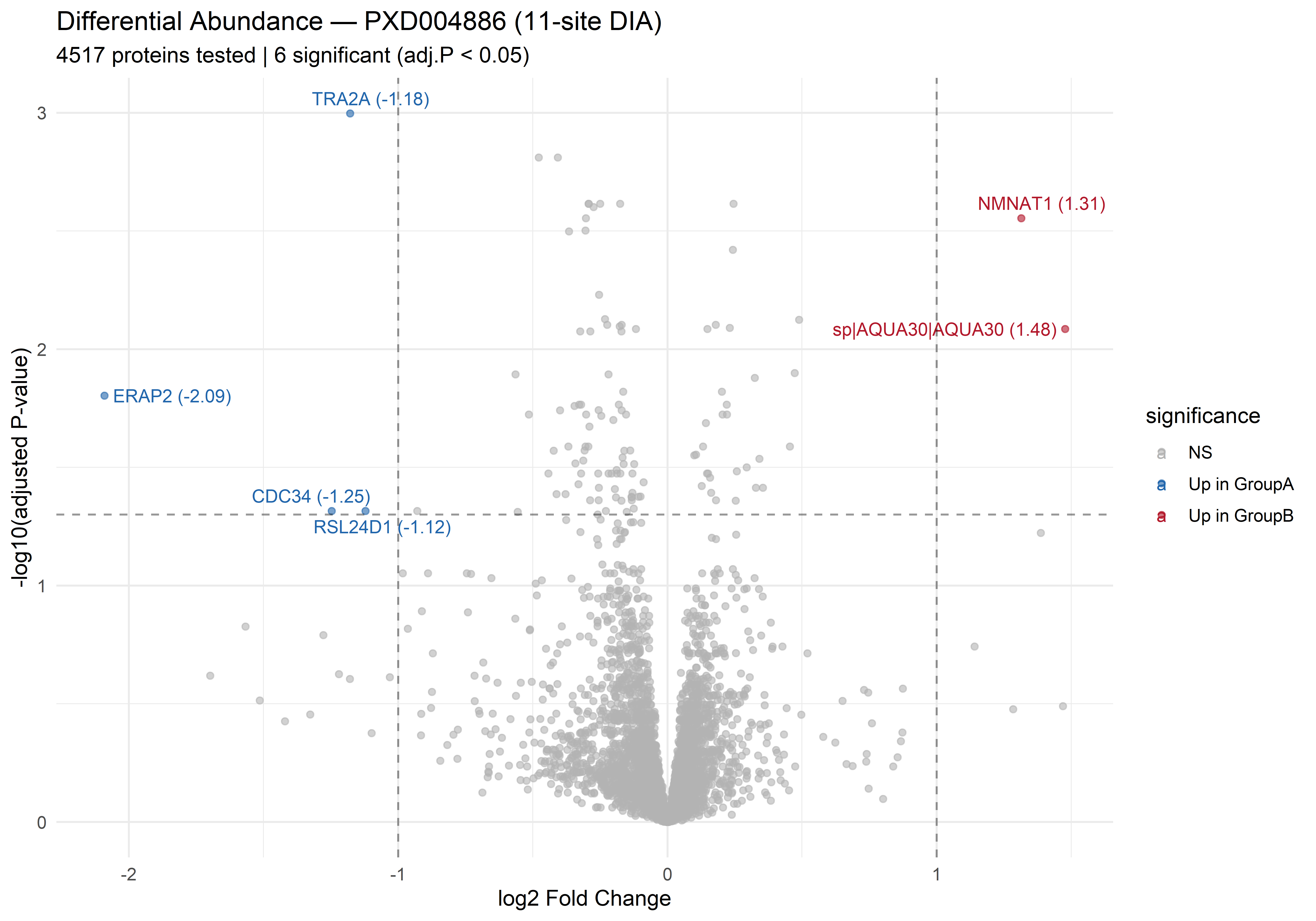
| Gene | log2FC | Adj. P | Direction | Biological Context |
|---|---|---|---|---|
| TRA2A | −1.18 | 0.001 | Group A ↑ | Transformer-2 alpha — splicing regulator; elevated in certain cancers |
| NMNAT1 | +1.31 | 0.003 | Group B ↑ | NAD+ biosynthesis enzyme; neuroprotective in Wallerian degeneration |
| AQUA30 | +1.48 | 0.008 | Group B ↑ | Spike-in standard — positive control confirming DE pipeline works |
| ERAP2 | −2.09 | 0.016 | Group A ↑ | Endoplasmic reticulum aminopeptidase 2 — antigen processing |
| CDC34 | −1.25 | 0.048 | Group A ↑ | Ubiquitin-conjugating enzyme — cell cycle regulation |
| RSL24D1 | −1.12 | 0.048 | Group A ↑ | Ribosomal protein — translational control |
The detection of AQUA30 as significantly differentially abundant (log2FC = +1.48, adj. P = 0.008) is the most important result: as a spike-in standard spiked at known concentration in Group B samples, its detection confirms that the entire pipeline — from peptide detection through normalisation to statistical testing — is functioning correctly. If AQUA30 were not significant, we would suspect a problem with the data processing before interpreting any biological hits.
CON__), decoys (REV__), and spike-ins if present.prcomp() — does PC1 separate samples by biological group or by batch?limma with an appropriate design matrix for your experimental design.library(DEP)
data("UbiLength")
# Inspect
dim(UbiLength)
colnames(UbiLength)[1:10]
# Identify intensity columns
int_cols <- grep("^LFQ", colnames(UbiLength), value = TRUE)
cat("Intensity columns:", length(int_cols), "\n")ubi_clean <- UbiLength |>
filter(
!grepl("^REV__", Gene.names),
!grepl("^CON__", Gene.names),
Potential.contaminant != "+"
)
cat("Proteins after filtering:", nrow(ubi_clean), "\n")Main output: filtered LFQ table.
miss_mat <- ubi_clean[, int_cols] |>
  as.matrix() |>
  log2()

miss_mat[is.infinite(miss_mat)] <- NA

frac_missing <- apply(miss_mat, 1, function(x) mean(is.na(x)))

ggplot(data.frame(frac_missing), aes(frac_missing)) +
  geom_histogram(bins = 30, fill = "#4682B4", colour = "white") +
  labs(title = "Protein-level missingness", x = "Fraction missing", y = "Count") +
  theme_minimal()
Main output: missingness plot.
# Log2 transform
log2_mat <- log2(as.matrix(ubi_clean[, int_cols]))
log2_mat[is.infinite(log2_mat)] <- NA

# Median centering
med_norm <- sweep(log2_mat, 2, apply(log2_mat, 2, median, na.rm = TRUE), "-")

# Cyclic loess (limma)
loess_norm <- normalizeCyclicLoess(log2_mat, method = "fast")

# Before / after density
plot_density <- function(mat, title) {
  df <- as.data.frame(mat) |>
    tidyr::pivot_longer(everything(), names_to = "sample", values_to = "intensity")
  ggplot(df, aes(intensity, colour = sample)) +
    geom_density(show.legend = FALSE) +
    labs(title = title, x = "log2 intensity") +
    theme_minimal()
}

plot_density(log2_mat, "Before normalization") +
plot_density(med_norm, "After median normalization")
Main output: normalized peptide matrix + before/after density plots.
# Median summarization
protein_median <- apply(med_norm, 1, median, na.rm = TRUE)

# Robust summarization via MsCoreUtils
protein_robust <- MsCoreUtils::robustSummary(med_norm)

# Comparison plot
comparison_df <- data.frame(
  median = protein_median,
  robust = protein_robust
)

ggplot(comparison_df, aes(median, robust)) +
  geom_point(alpha = 0.4, size = 0.8) +
  geom_abline(slope = 1, intercept = 0, colour = "red", linetype = "dashed") +
  labs(title = "Median vs robust protein summarization",
       x = "Median summarization (log2)",
       y = "Robust summarization (log2)") +
  theme_minimal()
Main output: protein abundance matrix + median vs robust comparison.
pca_plot <- function(mat, title, coldata) {
  complete_rows <- complete.cases(mat)
  pca <- prcomp(t(mat[complete_rows, ]), scale. = TRUE)
  df  <- as.data.frame(pca$x[, 1:2])
  df$condition <- coldata
  ggplot(df, aes(PC1, PC2, colour = condition)) +
    geom_point(size = 3) +
    labs(title = title) +
    theme_minimal()
}

# TODO: replace with actual condition metadata
condition <- rep(c("Control", "Treatment"), each = ncol(med_norm) / 2)

pca_plot(med_norm,   "PCA: Peptide level", condition) +
pca_plot(protein_robust |> matrix(nrow = 1), "PCA: Protein level", condition)
Main output: PCA at peptide and protein levels.
protein_report <- ubi_clean |>
  select(Gene.names, Protein.IDs) |>
  mutate(
    n_peptides      = rowSums(!is.na(med_norm)),
    median_abundance = protein_median,
    robust_abundance = protein_robust
  )

write.csv(protein_report, "results/lfq_protein_report.csv", row.names = FALSE)
Main output: protein quantification report.
An alternative to the DEP + limma workflow shown here is MSstats, which operates at the peptide- or transition-level with linear mixed models and performs protein-level inference as part of the test rather than as a separate aggregation step. See Chapter 12 for a full overview of the MSstats ecosystem, including MSstatsTMT, MSstatsPTM, MSstatsConvert, and related packages.
| Output | Description |
|---|---|
| Filtered LFQ table | Contaminants and reverse hits removed |
| Missingness plot | Per-protein fraction of missing values |
| Normalized peptide matrix | Median- and loess-normalized intensities |
| Protein abundance matrix | One row per protein group |
| Summarization comparison | Median vs robust aggregation differences |
| PCA plots | Peptide- and protein-level sample clustering |
| Protein quantification report | CSV ready for Programs 15–17 |
UbiLength dataset from DEP, compare the number of proteins retained when requiring ≥ 2 valid values in (a) all samples, (b) at least one condition group. Which strategy is more appropriate for a two-group comparison and why?MsCoreUtils::robustSummary and median. Identify three proteins whose abundance estimates differ by more than 20% between methods. What characteristics (number of peptides, missingness pattern) predict disagreement?sessioninfo::session_info()