12 Build and Audit a Quantitative Proteomics Data Object

You cannot measure a protein directly. You measure peptides, then argue your way up to the protein — propagating every filtering decision and every missing value as you go. Get that bookkeeping wrong and a “differentially abundant protein” can be an artifact of which peptides you happened to keep. This chapter builds the QFeatures object that keeps the PSM → peptide → protein hierarchy honest, linked, and auditable.

The One Mistake to Avoid

Aggregating peptides to proteins before filtering. Summarizing over contaminants, one-hit-wonders, and mostly-missing peptides bakes noise straight into the protein value. Filter first, then aggregate.

12.1 Learning Objectives

By the end of this chapter you will be able to:

Describe how QFeatures organises the PSM → peptide → protein hierarchy
Import quantitative proteomics data and construct a QFeatures object
Filter, log-transform, normalize, and aggregate features across levels
Diagnose data quality with PCA and missing-value visualisation
Run a basic differential test and compare standard versus robust aggregation

12.2 Understanding Quantitative MS Data

12.2.1 Quantitation Methodologies

There are several approaches to quantitative proteomics, each with distinct advantages:

Code

library(QFeatures)
library(tidyverse)
library(limma)
library(ggplot2)
library(pheatmap)

factoextra_available <- suppressWarnings(requireNamespace("factoextra", quietly = TRUE))

Label-free MS1: Extracted Ion Chromatograms (XIC)

In label-free quantitation, precursor peaks matching identified peptides are integrated over retention time.

Labelled MS2: Isobaric Tagging (TMT/iTRAQ)

Isobaric tags allow multiplexed quantitation where peptides from different samples are chemically labeled and analyzed together.

Label-free MS2: Spectral Counting

Simple counting of peptide-spectrum matches assigned to each protein.

Labelled MS1: SILAC

Stable isotope labeling allows direct comparison between heavy and light labeled samples.

12.3 The QFeatures Framework

12.3.1 QFeatures Class Structure

QFeatures extends the MultiAssayExperiment class to handle the hierarchical nature of MS data (spectra → peptides → proteins).

Code

flowchart TD
    subgraph QF["QFeatures Object Structure"]
        direction TB
        A[QFeatures Container] --> B[colData<br/>Sample Metadata]
        A --> C[Assays<br/>Hierarchical Levels]
        A --> D[rowData<br/>Feature Annotations]
        
        C --> E1[PSMs Assay<br/>Rows: 5000 PSMs<br/>Cols: 10 Samples]
        C --> E2[Peptides Assay<br/>Rows: 2500 Peptides<br/>Cols: 10 Samples]
        C --> E3[Proteins Assay<br/>Rows: 800 Proteins<br/>Cols: 10 Samples]
        
        E1 -->|aggregateFeatures<br/>by Sequence| E2
        E2 -->|aggregateFeatures<br/>by Protein| E3
    end
    
    subgraph Meta["Metadata Propagation"]
        F[Sample Info<br/>Condition, Batch, etc.] --> B
        G1[PSM Annotations<br/>Scores, RT, m/z] --> D
        G2[Peptide Info<br/>Sequence, Modifications] --> D
        G3[Protein Info<br/>Accession, Gene] --> D
    end
    
    subgraph Process["Data Processing"]
        E3 --> H[filterNA<br/>Remove Missing]
        H --> I[normalize<br/>Median/Quantile]
        I --> J[impute<br/>KNN/MinProb]
        J --> K[logTransform<br/>log2]
        K --> L[limma Analysis<br/>Differential Expression]
    end
    
  style QF fill:#D7E6FB,stroke:#27408B,stroke-width:3px,color:#102A43
  style Meta fill:#FBE0FA,stroke:#B000B0,stroke-width:3px,color:#102A43
  style Process fill:#D7E6FB,stroke:#27408B,stroke-width:3px,color:#102A43

flowchart TD
    subgraph QF["QFeatures Object Structure"]
        direction TB
        A[QFeatures Container] --> B[colData<br/>Sample Metadata]
        A --> C[Assays<br/>Hierarchical Levels]
        A --> D[rowData<br/>Feature Annotations]
        
        C --> E1[PSMs Assay<br/>Rows: 5000 PSMs<br/>Cols: 10 Samples]
        C --> E2[Peptides Assay<br/>Rows: 2500 Peptides<br/>Cols: 10 Samples]
        C --> E3[Proteins Assay<br/>Rows: 800 Proteins<br/>Cols: 10 Samples]
        
        E1 -->|aggregateFeatures<br/>by Sequence| E2
        E2 -->|aggregateFeatures<br/>by Protein| E3
    end
    
    subgraph Meta["Metadata Propagation"]
        F[Sample Info<br/>Condition, Batch, etc.] --> B
        G1[PSM Annotations<br/>Scores, RT, m/z] --> D
        G2[Peptide Info<br/>Sequence, Modifications] --> D
        G3[Protein Info<br/>Accession, Gene] --> D
    end
    
    subgraph Process["Data Processing"]
        E3 --> H[filterNA<br/>Remove Missing]
        H --> I[normalize<br/>Median/Quantile]
        I --> J[impute<br/>KNN/MinProb]
        J --> K[logTransform<br/>log2]
        K --> L[limma Analysis<br/>Differential Expression]
    end
    
  style QF fill:#D7E6FB,stroke:#27408B,stroke-width:3px,color:#102A43
  style Meta fill:#FBE0FA,stroke:#B000B0,stroke-width:3px,color:#102A43
  style Process fill:#D7E6FB,stroke:#27408B,stroke-width:3px,color:#102A43

QFeatures Advantages

Traceability: Links between PSMs, peptides, and proteins maintained throughout
Flexibility: Multiple assays can coexist (different processing strategies)
Metadata: Sample and feature annotations travel with the data
Reproducibility: Complete processing pipeline encoded in object

Code

# Load example data
data(feat1)
feat1

An instance of class QFeatures containing 1 set(s):
 [1] psms: SummarizedExperiment with 10 rows and 2 columns

Code

# Examine the structure
colData(feat1)

DataFrame with 2 rows and 1 column
       Group
   <integer>
S1         1
S2         2

Code

# Access the PSM-level assay
psms_assay <- feat1[["psms"]]
psms_assay

class: SummarizedExperiment 
dim: 10 2 
metadata(0):
assays(1): ''
rownames(10): PSM1 PSM2 ... PSM9 PSM10
rowData names(5): Sequence Protein Var location pval
colnames(2): S1 S2
colData names(0):

Code

# View quantitative data
assay(psms_assay)

      S1 S2
PSM1   1 11
PSM2   2 12
PSM3   3 13
PSM4   4 14
PSM5   5 15
PSM6   6 16
PSM7   7 17
PSM8   8 18
PSM9   9 19
PSM10 10 20

Code

# Examine row annotations
rowData(psms_assay)

DataFrame with 10 rows and 5 columns
           Sequence     Protein       Var      location      pval
        <character> <character> <integer>   <character> <numeric>
PSM1       SYGFNAAR       ProtA         1 Mitochondr...     0.084
PSM2       SYGFNAAR       ProtA         2 Mitochondr...     0.077
PSM3       SYGFNAAR       ProtA         3 Mitochondr...     0.063
PSM4       ELGNDAYK       ProtA         4 Mitochondr...     0.073
PSM5       ELGNDAYK       ProtA         5 Mitochondr...     0.012
PSM6       ELGNDAYK       ProtA         6 Mitochondr...     0.011
PSM7  IAEESNFPFI...       ProtB         7       unknown     0.075
PSM8  IAEESNFPFI...       ProtB         8       unknown     0.038
PSM9  IAEESNFPFI...       ProtB         9       unknown     0.028
PSM10 IAEESNFPFI...       ProtB        10       unknown     0.097

12.3.2 Feature Aggregation

A key feature of QFeatures is the ability to aggregate features from lower to higher levels while maintaining traceability.

Code

# Aggregate PSMs to peptides based on sequence
feat1 <- aggregateFeatures(feat1, 
                          i = "psms",
                          fcol = "Sequence", 
                          name = "peptides",
                          fun = colMeans)
feat1

An instance of class QFeatures containing 2 set(s):
 [1] psms: SummarizedExperiment with 10 rows and 2 columns 
 [2] peptides: SummarizedExperiment with 3 rows and 2 columns

Code

# Examine the peptide-level data
assay(feat1[["peptides"]])

             S1   S2
ELGNDAYK    5.0 15.0
IAEESNFPFIK 8.5 18.5
SYGFNAAR    2.0 12.0

Code

# Check aggregation statistics
rowData(feat1[["peptides"]])

DataFrame with 3 rows and 4 columns
                 Sequence     Protein      location        .n
              <character> <character>   <character> <integer>
ELGNDAYK         ELGNDAYK       ProtA Mitochondr...         3
IAEESNFPFIK IAEESNFPFI...       ProtB       unknown         4
SYGFNAAR         SYGFNAAR       ProtA Mitochondr...         3

Code

# Aggregate peptides to proteins
feat1 <- aggregateFeatures(feat1,
                          i = "peptides", 
                          fcol = "Protein",
                          name = "proteins",
                          fun = colMedians)
feat1

An instance of class QFeatures containing 3 set(s):
 [1] psms: SummarizedExperiment with 10 rows and 2 columns 
 [2] peptides: SummarizedExperiment with 3 rows and 2 columns 
 [3] proteins: SummarizedExperiment with 2 rows and 2 columns

Code

# View final protein quantification
assay(feat1[["proteins"]])

       S1   S2
ProtA 3.5 13.5
ProtB 8.5 18.5

12.3.3 Subsetting and Filtering

QFeatures maintains relationships between assays during subsetting operations.

Code

# Subset for a specific protein
protein_a <- feat1["ProtA", , ]
protein_a

An instance of class QFeatures containing 3 set(s):
 [1] psms: SummarizedExperiment with 6 rows and 2 columns 
 [2] peptides: SummarizedExperiment with 2 rows and 2 columns 
 [3] proteins: SummarizedExperiment with 1 rows and 2 columns

Code

# Filter features based on quality criteria
feat1_filtered <- filterFeatures(feat1, ~ pval < 0.05)
feat1_filtered

An instance of class QFeatures containing 3 set(s):
 [1] psms: SummarizedExperiment with 4 rows and 2 columns 
 [2] peptides: SummarizedExperiment with 0 rows and 2 columns 
 [3] proteins: SummarizedExperiment with 0 rows and 2 columns

12.4 Working with Real Data: CPTAC Dataset

12.4.1 Data Import

Code

library(MsDataHub)

# Load CPTAC peptide data
# Note: This is a simulated example based on the CPTAC study design
set.seed(123)

# Create sample metadata
sample_info <- data.frame(
  sample = paste0("Sample_", 1:6),
  condition = rep(c("6A", "6B"), each = 3),
  replicate = rep(1:3, 2),
  row.names = paste0("Sample_", 1:6)
)

# Simulate peptide quantification data
n_peptides <- 1000
peptide_data <- matrix(
  rlnorm(n_peptides * 6, meanlog = 10, sdlog = 1),
  nrow = n_peptides,
  ncol = 6,
  dimnames = list(
    paste0("Peptide_", 1:n_peptides),
    rownames(sample_info)
  )
)

# Add differential expression signal
de_peptides <- 1:100  # First 100 peptides are differentially expressed
peptide_data[de_peptides, 4:6] <- peptide_data[de_peptides, 4:6] * 1.5

# Create row annotations
peptide_annotations <- data.frame(
  Sequence = paste0("SEQ", 1:n_peptides),
  Proteins = sample(paste0("PROT", 1:200), n_peptides, replace = TRUE),
  PEP = runif(n_peptides, 0, 0.1),
  Score = runif(n_peptides, 20, 100),
  row.names = rownames(peptide_data)
)

# Create SummarizedExperiment
library(SummarizedExperiment)
cptac_se <- SummarizedExperiment(
  assays = list(peptides = peptide_data),
  rowData = peptide_annotations,
  colData = sample_info
)

# Create QFeatures object
cptac_qf <- QFeatures(list(peptides = cptac_se))
cptac_qf

An instance of class QFeatures containing 1 set(s):
 [1] peptides: SummarizedExperiment with 1000 rows and 6 columns

12.4.2 Data Preprocessing Pipeline

Code

# Log transformation
cptac_qf <- logTransform(cptac_qf, 
                        i = "peptides",
                        name = "log_peptides")

# Normalization (median centering)
cptac_qf <- normalize(cptac_qf,
                     i = "log_peptides", 
                     name = "norm_peptides",
                     method = "center.median")

cptac_qf

An instance of class QFeatures containing 3 set(s):
 [1] peptides: SummarizedExperiment with 1000 rows and 6 columns 
 [2] log_peptides: SummarizedExperiment with 1000 rows and 6 columns 
 [3] norm_peptides: SummarizedExperiment with 1000 rows and 6 columns

12.4.3 Missing Value Analysis

Code

# Introduce some missing values for demonstration
assay_data <- assay(cptac_qf[["norm_peptides"]])
# Set 10% of values to NA randomly
missing_indices <- sample(length(assay_data), length(assay_data) * 0.1)
assay_data[missing_indices] <- NA
assay(cptac_qf[["norm_peptides"]]) <- assay_data

# Analyze missing value patterns
na_stats <- nNA(cptac_qf[["norm_peptides"]])
cat("Overall missing values:", na_stats$nNA$pNA * 100, "%\n")

Overall missing values: 10 %

Code

# Visualize missing value patterns
missing_pattern <- na_stats$nNArows
head(missing_pattern, 10)

DataFrame with 10 rows and 3 columns
          name       nNA       pNA
   <character> <integer> <numeric>
1    Peptide_1         1  0.166667
2    Peptide_2         2  0.333333
3    Peptide_3         1  0.166667
4    Peptide_4         2  0.333333
5    Peptide_5         2  0.333333
6    Peptide_6         1  0.166667
7    Peptide_7         1  0.166667
8    Peptide_8         0  0.000000
9    Peptide_9         1  0.166667
10  Peptide_10         0  0.000000

Code

# Filter peptides with too many missing values
cptac_qf_clean <- filterNA(cptac_qf, i = "norm_peptides", pNA = 0.5)
cat("Peptides after filtering:", nrow(cptac_qf_clean[["norm_peptides"]]), "\n")

Peptides after filtering: 1000

12.4.4 Protein Aggregation

Code

# Aggregate to protein level using median
cptac_qf_clean <- aggregateFeatures(cptac_qf_clean,
                                   i = "norm_peptides",
                                   fcol = "Proteins", 
                                   name = "proteins",
                                   fun = colMedians,
                                   na.rm = TRUE)

cptac_qf_clean

An instance of class QFeatures containing 4 set(s):
 [1] peptides: SummarizedExperiment with 1000 rows and 6 columns 
 [2] log_peptides: SummarizedExperiment with 1000 rows and 6 columns 
 [3] norm_peptides: SummarizedExperiment with 1000 rows and 6 columns 
 [4] proteins: SummarizedExperiment with 197 rows and 6 columns

Code

# Examine aggregation results
aggregation_stats <- rowData(cptac_qf_clean[["proteins"]])[".n"]
table(aggregation_stats)

.n
 1  2  3  4  5  6  7  8  9 10 11 13 14 
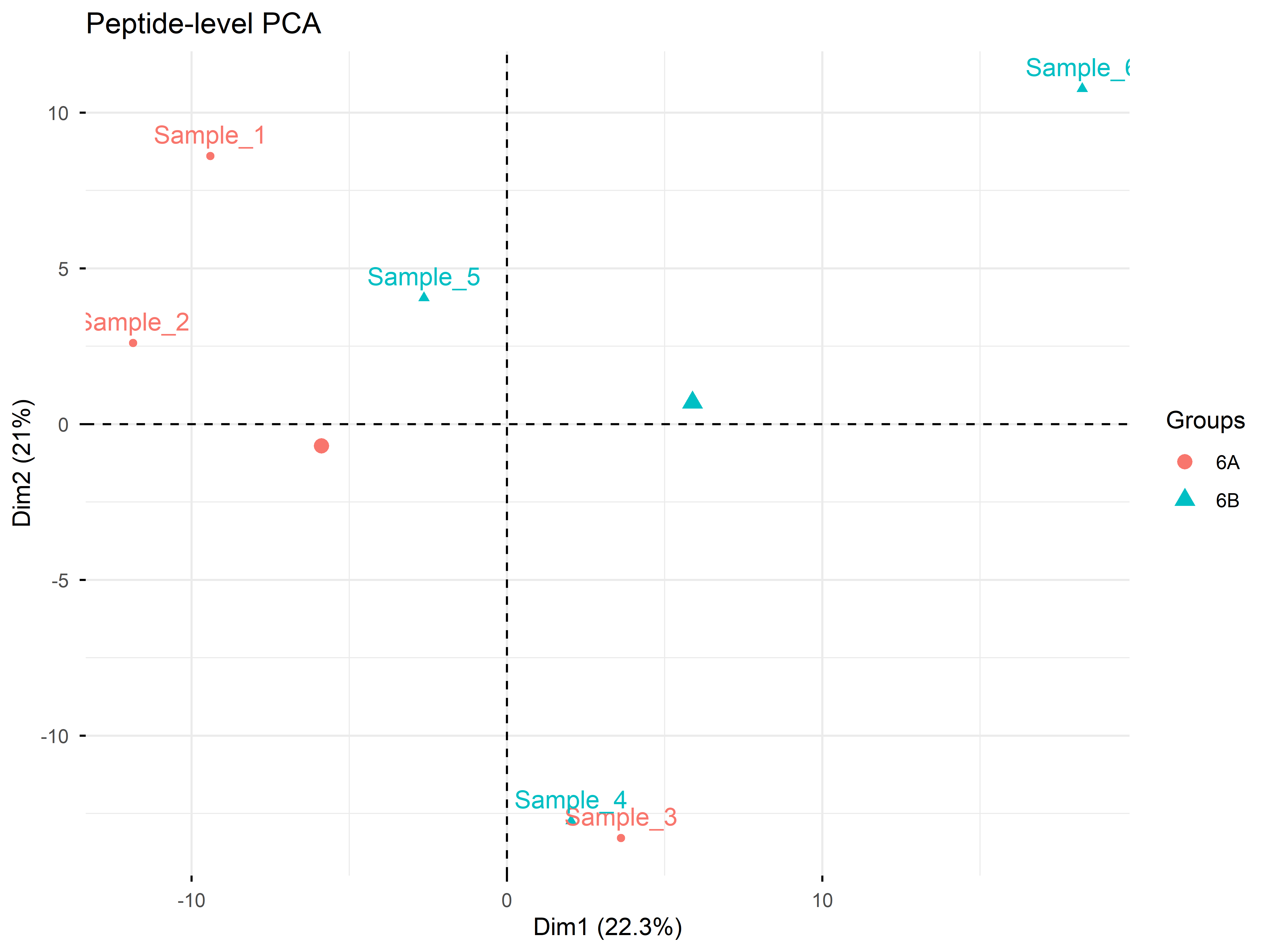
 6 16 27 42 32 28 18 13  6  5  1  2  1

12.5 Quality Control and Visualization

12.5.1 Principal Component Analysis

Code

# PCA on peptide-level data
peptide_pca <- cptac_qf_clean[["norm_peptides"]] %>%
  filterNA() %>%
  assay() %>%
  t() %>%
  prcomp(scale = TRUE, center = TRUE)

# Create PCA plot
if (factoextra_available) {
  factoextra::fviz_pca_ind(
    peptide_pca,
    habillage = colData(cptac_qf_clean)$condition,
    title = "Peptide-level PCA"
  )
} else {
  peptide_scores <- as.data.frame(peptide_pca$x[, 1:2])
  peptide_scores$condition <- colData(cptac_qf_clean)$condition

  ggplot(peptide_scores, aes(x = PC1, y = PC2, color = condition)) +
    geom_point(size = 3, alpha = 0.8) +
    labs(title = "Peptide-level PCA") +
    theme_minimal()
}

Code

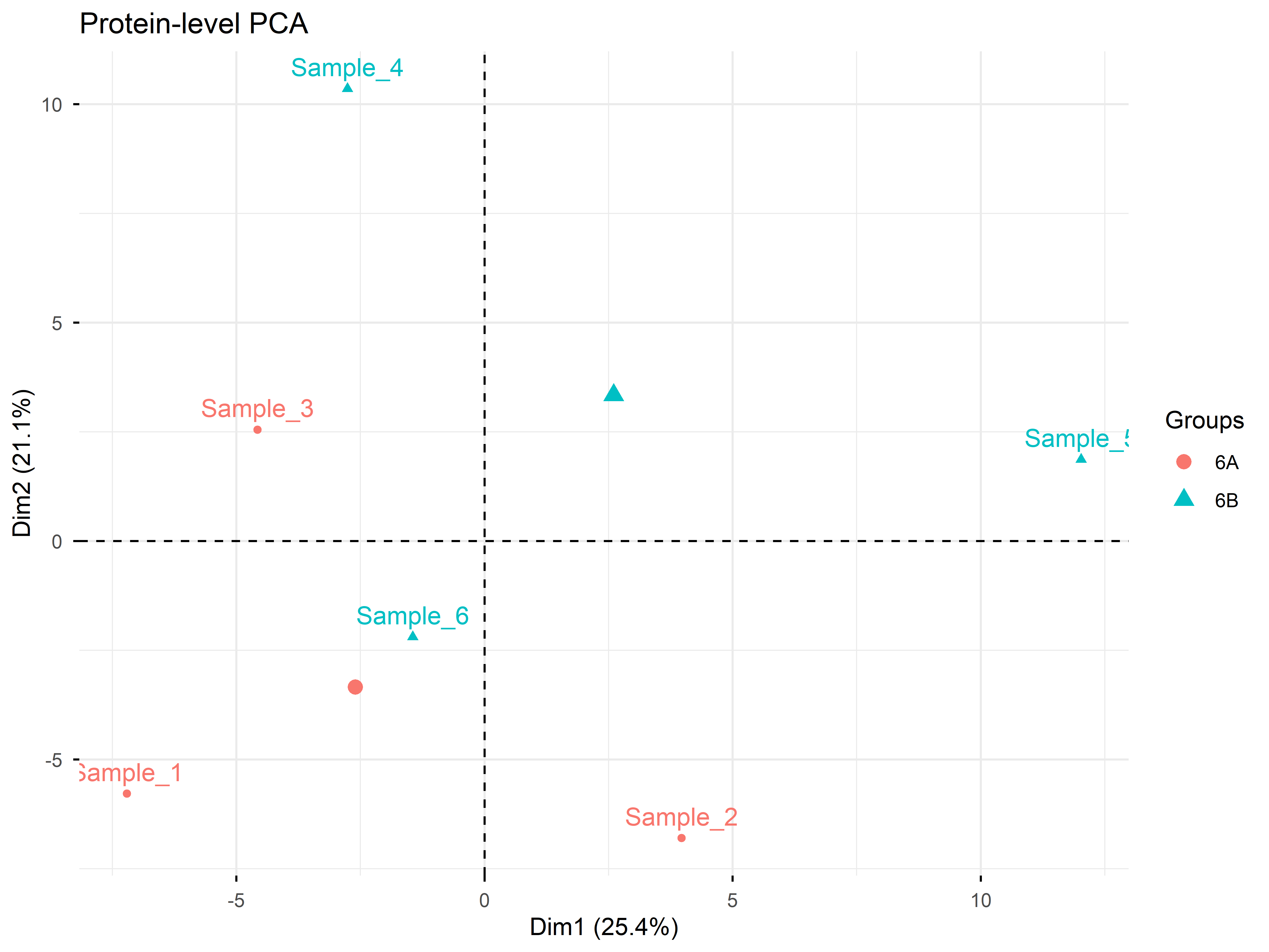
# PCA on protein-level data  
protein_pca <- cptac_qf_clean[["proteins"]] %>%
  filterNA() %>%
  assay() %>%
  t() %>%
  prcomp(scale = TRUE, center = TRUE)

if (factoextra_available) {
  factoextra::fviz_pca_ind(
    protein_pca,
    habillage = colData(cptac_qf_clean)$condition,
    title = "Protein-level PCA"
  )
} else {
  protein_scores <- as.data.frame(protein_pca$x[, 1:2])
  protein_scores$condition <- colData(cptac_qf_clean)$condition

  ggplot(protein_scores, aes(x = PC1, y = PC2, color = condition)) +
    geom_point(size = 3, alpha = 0.8) +
    labs(title = "Protein-level PCA") +
    theme_minimal()
}

12.5.2 Expression Profile Visualization

Code

# Extract data for a specific protein using longForm
example_protein <- rownames(assay(cptac_qf_clean[["proteins"]]))[1]

profile_data <- longForm(cptac_qf_clean[example_protein, , 
                                       c("norm_peptides", "proteins")]) %>%
  as_tibble()

# Get column data and ensure unique column names
col_data <- as_tibble(colData(cptac_qf_clean), rownames = "sample_id")

# Join the data
profile_data <- profile_data %>%
  left_join(col_data, by = c("colname" = "sample_id"))

ggplot(profile_data, aes(x = colname, y = value, color = condition)) +
  geom_point(size = 3) +
  geom_line(aes(group = rowname)) +
  facet_wrap(~assay, scales = "free_y") +
  theme_minimal() +
  theme(axis.text.x = element_text(angle = 45, hjust = 1)) +
  labs(title = paste("Expression Profile:", example_protein),
       x = "Sample", y = "Normalized Intensity")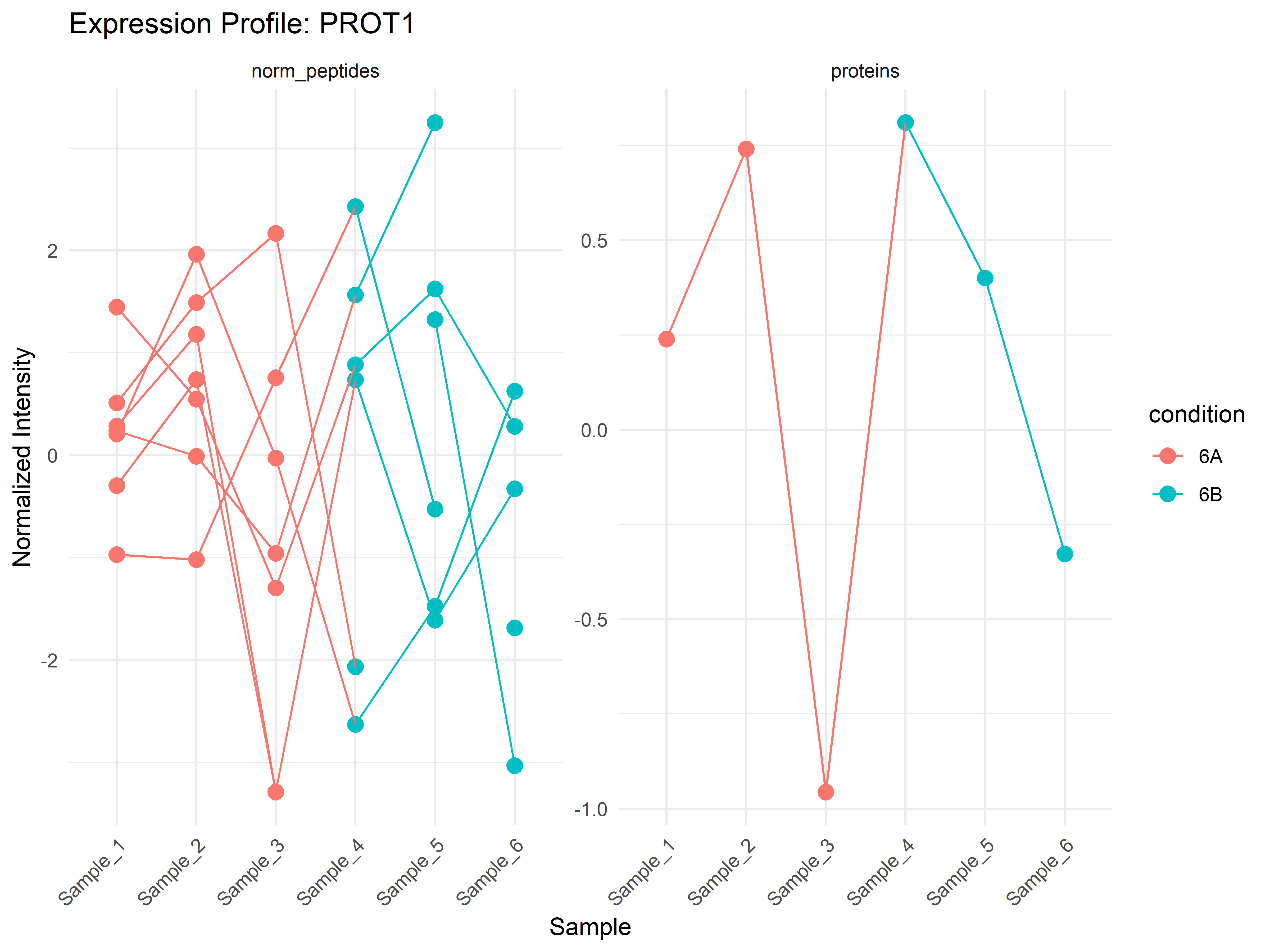

12.6 Statistical Analysis

12.6.1 Differential Expression with limma

Code

# Extract protein data for statistical analysis
protein_data <- getWithColData(cptac_qf_clean, "proteins")

# Set up design matrix
design <- model.matrix(~ condition, data = colData(protein_data))
colnames(design) <- c("Intercept", "Condition_6B_vs_6A")

# Fit linear model
fit <- lmFit(assay(protein_data), design)
fit <- eBayes(fit)

# Extract results
results <- topTable(fit, coef = "Condition_6B_vs_6A", number = Inf) %>%
  rownames_to_column("protein") %>%
  as_tibble()

head(results)

# A tibble: 6 × 7
  protein logFC AveExpr     t P.Value adj.P.Val     B
  <chr>   <dbl>   <dbl> <dbl>   <dbl>     <dbl> <dbl>
1 PROT157 -2.27   0.226 -3.88 0.00153     0.301 -1.33
2 PROT137 -1.83   0.372 -3.24 0.00558     0.549 -2.22
3 PROT140  1.70   0.859  2.94 0.0102      0.650 -2.64
4 PROT188 -1.84  -0.551 -2.77 0.0144      0.650 -2.88
5 PROT78   1.51  -0.224  2.71 0.0165      0.650 -2.97
6 PROT187  1.93   0.220  2.46 0.0277      0.824 -3.36

Code

# Volcano plot
results %>%
  ggplot(aes(x = logFC, y = -log10(P.Value))) +
  geom_point(alpha = 0.6) +
  geom_hline(yintercept = -log10(0.05), linetype = "dashed", color = "red") +
  geom_vline(xintercept = c(-1, 1), linetype = "dashed", color = "red") +
  labs(title = "Volcano Plot",
       x = "log2 Fold Change", 
       y = "-log10 P-value") +
  theme_minimal()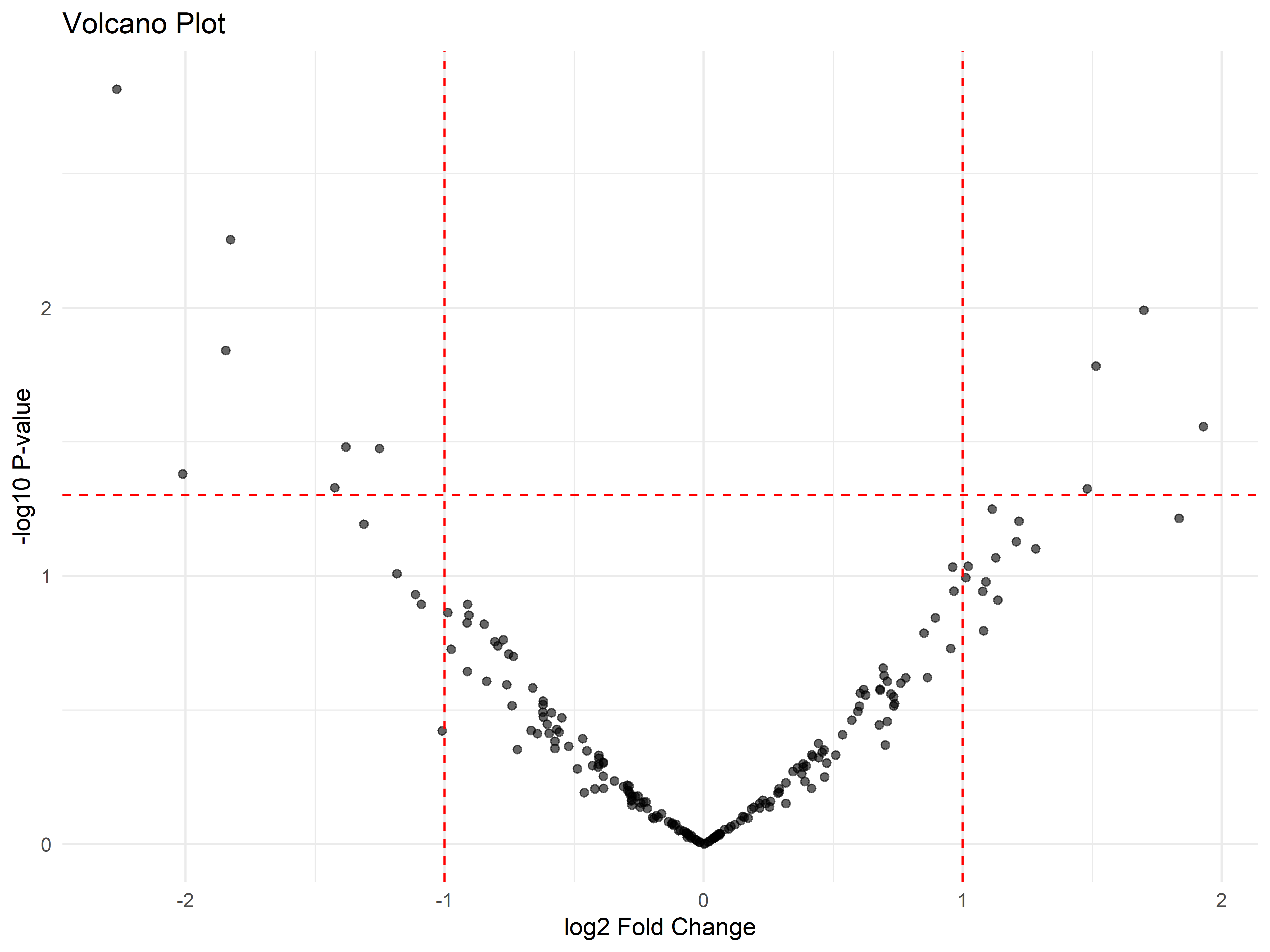

Code

# Summary of differential expression
significant_proteins <- results %>%
  filter(adj.P.Val < 0.05, abs(logFC) > 1)

cat("Significantly changed proteins:", nrow(significant_proteins), "\n")

Significantly changed proteins: 0

Code

cat("Up-regulated:", sum(significant_proteins$logFC > 1), "\n")

Up-regulated: 0

Code

cat("Down-regulated:", sum(significant_proteins$logFC < -1), "\n")

Down-regulated: 0

12.6.2 Heatmap of Significant Proteins

Code

if (nrow(significant_proteins) > 5) {
  # Select top 20 most significant proteins
  top_proteins <- head(significant_proteins, 20)$protein
  
  # Create heatmap data
  heatmap_data <- assay(protein_data)[top_proteins, ]
  
  # Sample annotations
  annotation_col <- data.frame(
    Condition = colData(protein_data)$condition,
    row.names = colnames(heatmap_data)
  )
  
  # Generate heatmap
  pheatmap(heatmap_data,
           annotation_col = annotation_col,
           scale = "row",
           clustering_distance_rows = "euclidean",
           clustering_distance_cols = "euclidean",
           main = "Top Differentially Expressed Proteins")
}

12.7 Where MSstats Fits

The workflow above stays within the Bioconductor QFeatures ecosystem: limma operates on the protein-level matrix produced by aggregateFeatures(). An alternative ecosystem, MSstats, approaches quantification from the opposite direction – it models peptide- or transition-level intensities directly, using linear mixed models, and performs protein-level inference as part of the statistical test rather than as a separate aggregation step.

12.7.1 The MSstats Family

The MSstats ecosystem has grown into a family of specialised packages, each tailored to a specific input type and experimental design:

Package	Input	Purpose
MSstats	Peptide- or transition-level intensities	Linear mixed models for label-free, DDA, DIA, and SRM; run-level summarisation with `dataProcess()` and differential testing with `groupComparison()`
MSstatsTMT	Reporter-ion intensities from TMT experiments	TMT-specific workflow: channel-level normalisation, purity correction, and protein-level inference across multiple TMT mixtures
MSstatsPTM	PTM + global (unmodified) protein abundances	Adjusts post-translational modification quantifications for changes in the parent protein abundance
MSstatsLiP	Limited proteolysis (LiP) data	Compares protease-accessible peptide profiles for structural proteomics
MSstatsConvert	Search-engine/vendor export files	Import and conversion layer: transforms output from DIA-NN, FragPipe, MaxQuant, Spectronaut, Skyline, and others into the MSstats-compatible format
MSstatsShiny	(GUI wrapper)	Point-and-click interface for interactive exploration; generates reproducible R scripts from the GUI session
MSstatsBig	Large-scale DIA datasets (>10 GB PSM files)	Handles datasets too large for in-memory processing via the `arrow` backend; pre-filters features before normalisation to reduce memory footprint

12.7.2 Standard MSstats Workflow

A typical MSstats analysis proceeds through four steps:

Import and convert — MSstatsConvert::MSstatsConvert() reads search-engine output and converts it to the standard MSstats format
Summarise — MSstats::dataProcess() performs run-level summarisation, normalisation, and missing-value handling
Compare — MSstats::groupComparison() fits linear mixed models and returns differential-abundance results
Visualise — MSstats::groupComparisonPlots() produces volcano plots, comparison plots, and heatmaps

Code

# Typical MSstats pipeline
library(MSstats)

# Convert search-engine output
# raw <- MSstatsConvert::MSstatsConvert(your_export_file)

# Process and summarise
# processed <- dataProcess(raw)

# Compare conditions
# comparison <- groupComparison(processed)

# Visualise
# groupComparisonPlots(comparison, type = "Volcano")

12.7.3 Version Sensitivity of Converters

The MSstatsConvert package is version-sensitive: different versions of search engines (MaxQuant, DIA-NN, FragPipe, Spectronaut, Skyline) may produce output formats that require specific converter versions. Always check the MSstats news and the converter vignette for the version compatibility table. If a converter fails, the first troubleshooting step is to update both the search engine and MSstatsConvert to their latest releases.

12.7.4 QFeatures vs MSstats: A Design Choice

The limma + QFeatures workflow demonstrated earlier in this chapter stays within the Bioconductor ecosystem. The MSstats family uses its own data structures and modelling framework. Both approaches are valid; the choice depends on your input format and desired model complexity:

Use QFeatures + limma when you want full control over each preprocessing step, need to integrate with other Bioconductor objects (SummarizedExperiment, MultiAssayExperiment), or prefer a separation of aggregation and testing.
Use MSstats when your data comes from search engines with native MSstats converters, you need peptide-level modelling with automatic protein-level inference, or you work with complex multi-factorial designs that benefit from the linear mixed model framework.

12.7.5 Exercises

Map three vendor/search-tool exports to the correct converter and downstream MSstats workflow: (a) MaxQuant proteinGroups.txt, (b) DIA-NN report.tsv, (c) Spectronaut xyz_Report.tsv.
Compare the output of MSstats::dataProcess() with the protein-level matrix produced by aggregateFeatures() — how do the summarised values differ?
Explain why MSstatsConvert version matters when working with a recently updated version of DIA-NN or FragPipe.

12.8 Advanced Aggregation Methods

12.8.1 Robust Summarization

Code

library(MsCoreUtils)

# Robust aggregation using robust summarization
cptac_robust <- aggregateFeatures(cptac_qf_clean,
                                 i = "norm_peptides",
                                 fcol = "Proteins",
                                 name = "proteins_robust", 
                                 fun = MsCoreUtils::robustSummary,
                                 na.rm = TRUE)

# Compare standard vs robust aggregation
comparison_data <- data.frame(
  standard = assay(cptac_qf_clean[["proteins"]])[, 1],
  robust = assay(cptac_robust[["proteins_robust"]])[, 1]
) %>%
  na.omit()

ggplot(comparison_data, aes(x = standard, y = robust)) +
  geom_point(alpha = 0.6) +
  geom_abline(slope = 1, intercept = 0, color = "red") +
  labs(title = "Standard vs Robust Aggregation",
       x = "Standard (Median)",
       y = "Robust Summarization") +
  theme_minimal()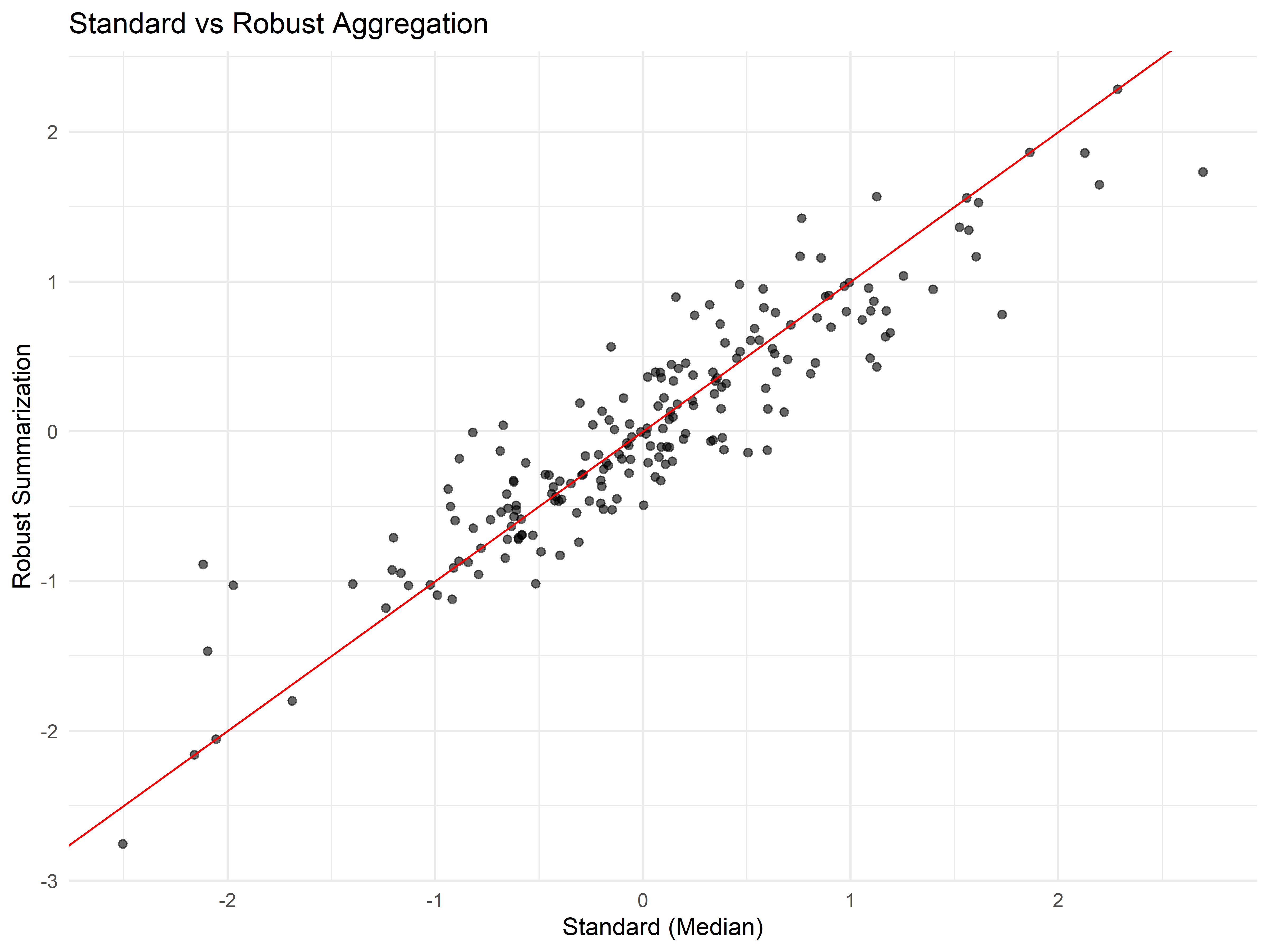

12.9 Working with QFeatures Workflows

12.9.1 Visualization of Data Relationships

Code

# Visualize the relationship between assays
plot(cptac_robust)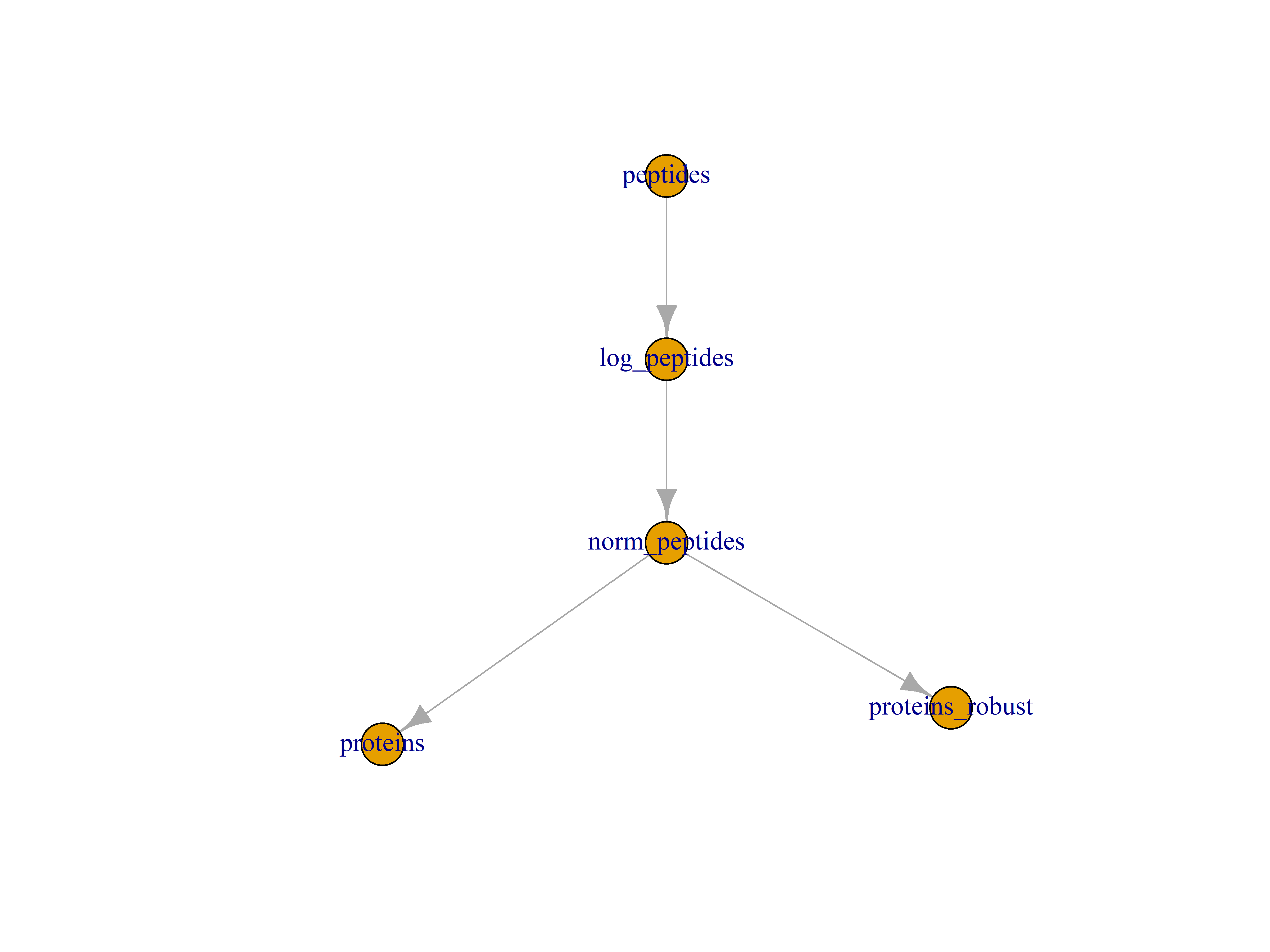

12.9.2 Custom Processing Functions

Code

# Example: Custom normalization using addAssay
quantile_normalize <- function(x) {
  # Simple quantile normalization implementation
  x_sorted <- apply(x, 2, sort, na.last = TRUE)
  x_mean <- rowMeans(x_sorted, na.rm = TRUE)
  
  for (i in 1:ncol(x)) {
    ranks <- rank(x[, i], na.last = "keep")
    x[, i] <- x_mean[ranks]
  }
  return(x)
}

# Apply custom normalization
log_peptides_se <- cptac_qf_clean[["log_peptides"]]
quantile_norm_assay <- quantile_normalize(assay(log_peptides_se))

# Create a new SummarizedExperiment with the normalized data
library(SummarizedExperiment)
quantile_norm_se <- SummarizedExperiment(
  assays = list(quantile_norm = quantile_norm_assay),
  rowData = rowData(log_peptides_se),
  colData = colData(log_peptides_se)
)

# Add to QFeatures object
cptac_custom <- addAssay(cptac_qf_clean,
                        quantile_norm_se,
                        name = "quantile_norm")

# Add assay link - for a transformation, use simple string-based linking
# This indicates that all features in quantile_norm come from log_peptides
cptac_custom <- addAssayLink(cptac_custom,
                            from = "log_peptides",
                            to = "quantile_norm")

cat("Custom normalization applied successfully\n")

Custom normalization applied successfully

Code

cat("Available assays:", names(cptac_custom), "\n")

Available assays: peptides log_peptides norm_peptides proteins quantile_norm

12.10 Exercises

Load the CPTAC dataset and perform complete preprocessing pipeline
Compare different aggregation methods (mean, median, robust)
Implement missing value imputation strategies
Perform differential expression analysis with multiple comparisons
Create custom visualization functions for QFeatures objects

12.11 Summary

This chapter introduced the QFeatures framework for quantitative proteomics analysis. Key concepts covered include:

Different quantitation methodologies in proteomics
The hierarchical structure of MS quantitative data
Feature aggregation strategies
Quality control and missing value handling
Statistical analysis workflows
Visualization of quantitative proteomics data

The QFeatures infrastructure provides a robust foundation for reproducible quantitative proteomics analysis in R.

12.12 Session Information

Code

sessionInfo()

R version 4.5.1 (2025-06-13 ucrt)
Platform: x86_64-w64-mingw32/x64
Running under: Windows 11 x64 (build 26200)

Matrix products: default
  LAPACK version 3.12.1

locale:
[1] LC_COLLATE=English_Switzerland.utf8  LC_CTYPE=English_Switzerland.utf8   
[3] LC_MONETARY=English_Switzerland.utf8 LC_NUMERIC=C                        
[5] LC_TIME=English_Switzerland.utf8    

time zone: Europe/Zurich
tzcode source: internal

attached base packages:
[1] stats4    stats     graphics  grDevices utils     datasets  methods  
[8] base     

other attached packages:
 [1] MsCoreUtils_1.20.0          MsDataHub_1.8.0            
 [3] pheatmap_1.0.13             limma_3.64.3               
 [5] lubridate_1.9.5             forcats_1.0.1              
 [7] stringr_1.6.0               dplyr_1.2.1                
 [9] purrr_1.2.2                 readr_2.2.0                
[11] tidyr_1.3.2                 tibble_3.3.1               
[13] ggplot2_4.0.3               tidyverse_2.0.0            
[15] QFeatures_1.18.0            MultiAssayExperiment_1.34.0
[17] SummarizedExperiment_1.38.1 Biobase_2.68.0             
[19] GenomicRanges_1.60.0        GenomeInfoDb_1.44.3        
[21] IRanges_2.42.0              S4Vectors_0.46.0           
[23] BiocGenerics_0.54.1         generics_0.1.4             
[25] MatrixGenerics_1.20.0       matrixStats_1.5.0          

loaded via a namespace (and not attached):
 [1] DBI_1.3.0               rlang_1.3.0             magrittr_2.0.5         
 [4] clue_0.3-68             otel_0.2.0              compiler_4.5.1         
 [7] RSQLite_3.53.3          png_0.1-9               vctrs_0.7.3            
[10] reshape2_1.4.5          ProtGenerics_1.40.0     pkgconfig_2.0.3        
[13] crayon_1.5.3            fastmap_1.2.0           backports_1.5.1        
[16] dbplyr_2.6.0            XVector_0.48.0          labeling_0.4.3         
[19] utf8_1.2.6              rmarkdown_2.31          tzdb_0.5.0             
[22] UCSC.utils_1.4.0        bit_4.6.0               xfun_0.60              
[25] cachem_1.1.0            jsonlite_2.0.0          blob_1.3.0             
[28] DelayedArray_0.34.1     broom_1.0.13            cluster_2.1.8.2        
[31] R6_2.6.1                stringi_1.8.7           RColorBrewer_1.1-3     
[34] car_3.1-5               Rcpp_1.1.2              knitr_1.51             
[37] BiocBaseUtils_1.10.0    Matrix_1.7-3            igraph_2.3.3           
[40] timechange_0.4.0        tidyselect_1.2.1        abind_1.4-8            
[43] yaml_2.3.12             curl_7.1.0              lattice_0.22-7         
[46] plyr_1.8.9              withr_3.0.3             KEGGREST_1.48.1        
[49] S7_0.2.2                evaluate_1.0.5          BiocFileCache_2.16.2   
[52] ExperimentHub_2.16.1    Biostrings_2.76.0       ggpubr_1.0.0           
[55] pillar_1.11.1           BiocManager_1.30.27     filelock_1.0.3         
[58] carData_3.0-6           BiocVersion_3.21.1      hms_1.1.4              
[61] scales_1.4.0            glue_1.8.1              lazyeval_0.2.3         
[64] tools_4.5.1             AnnotationHub_3.16.1    ggsignif_0.6.4         
[67] grid_4.5.1              AnnotationDbi_1.70.0    GenomeInfoDbData_1.2.14
[70] Formula_1.2-5           cli_3.6.5               rappdirs_0.3.4         
[73] S4Arrays_1.8.1          AnnotationFilter_1.32.0 gtable_0.3.6           
[76] rstatix_1.0.0           digest_0.6.37           SparseArray_1.8.1      
[79] ggrepel_0.9.8           htmlwidgets_1.6.4       farver_2.1.2           
[82] memoise_2.0.1           htmltools_0.5.9         factoextra_2.1.0       
[85] lifecycle_1.0.5         httr_1.4.8              statmod_1.5.2          
[88] bit64_4.8.2             MASS_7.3-65