# Detect Chromatographic Features with xcms
> *"A feature is just a number until you know which peaks from which samples agree that it is real."*
A raw LC–MS file is a haystack of millions of intensity readings. Buried inside are the few thousand chromatographic peaks that correspond to real molecules — and every result that follows depends on finding them faithfully, then finding them again in the same place across every sample. Set the detection parameters too loose and you drown in noise; too tight and you lose the biology. This chapter is the `xcms` pipeline that turns raw signal into a trustworthy feature matrix.
::: {.callout-warning title="The One Mistake to Avoid"}
Copying someone else's CentWave parameters. Peak-width and ppm depend on *your* chromatography and instrument; borrowed settings silently miss real peaks or invent noise ones. Tune them on your own QC samples.
:::
## Learning Objectives
By the end of this chapter you will be able to:
- Explain what a chromatographic **feature** is and how it differs from a raw spectral peak
- Configure and run **CentWave** peak detection with `findChromPeaks()`
- Diagnose poor parameter choices using peak count and signal-to-noise metrics
- Align retention times across samples with `adjustRtime()`
- Correspond peaks across samples into features with `groupChromPeaks()`
- Recover missed signal with `fillChromPeaks()` and export a quantitative feature matrix
------------------------------------------------------------------------
## What Is a Chromatographic Feature?
In untargeted LC-MS, the instrument acquires a full-scan mass spectrum every fraction of a second across the chromatographic run. The raw dataset is therefore two-dimensional: retention time × *m/z*. From this continuous surface we need to extract a compact, comparable representation — a **feature table** where each row is one compound and each column is one sample.
Two terms are important to keep distinct:
- A **chromatographic peak** is a locally elevated signal in a single sample at a specific *m/z* and retention time range. It corresponds to one compound eluting from the column in that run.
- A **feature** is the cross-sample correspondence: peaks from different runs that share the same *m/z* and (after alignment) the same retention time are grouped into a single feature. Features become the rows of your final intensity matrix.
The path from raw data to feature matrix follows four sequential steps:
```{mermaid}
%%| fig-width: 9
%%| fig-height: 3
flowchart LR
    A[Raw mzML\nSpectra] -->|findChromPeaks| B[Peaks per\nsample]
    B -->|adjustRtime| C[RT-aligned\npeaks]
    C -->|groupChromPeaks| D[Features across\nsamples]
    D -->|fillChromPeaks\n+ featureValues| E[Intensity\nmatrix]

    style A fill:#D7E6FB,stroke:#27408B
    style E fill:#ffffff,stroke:#27408B,stroke-width:2px
```
### The CentWave Triad: Three Parameters That Control Everything
The CentWave algorithm (`findChromPeaks` with `CentWaveParam`) detects chromatographic peaks by looking for regions of the *m/z*-RT plane where the signal exceeds a noise threshold. Three parameters dominate its behaviour:
| Parameter | What It Controls | Too Low | Too High |
|-----------|-----------------|---------|----------|
| **`ppm`** | m/z tolerance for grouping data points into a peak | Merges distinct peaks; inflated peak width | Splits real peaks; missed features |
| **`peakwidth`** | Expected chromatographic peak width range (seconds) | Picks up noise spikes; long computation | Misses narrow peaks |
| **`snthresh`** | Signal-to-noise ratio cutoff | Picks up noise; inflated feature count | Misses low-abundance features |
**The diagnostic principle:** After peak detection, always check:
1. **Number of peaks per sample** — should be roughly equal across samples. A sample with 10× fewer peaks than others has an injection or acquisition problem.
2. **Peak width distribution** — should be unimodal around your LC peak width (~10–60 s for UHPLC). Bimodal distributions suggest `peakwidth` is mis-specified.
3. **Peak density along retention time** — should be roughly uniform. Gaps indicate regions of poor chromatographic performance.
**Parameter tuning strategy for untargeted metabolomics:**
1. Start with `ppm = 15–30` for Q-TOF, `ppm = 5–10` for Orbitrap
2. Set `peakwidth = c(10, 60)` for UHPLC, `c(20, 120)` for HPLC
3. Set `snthresh = 10` initially; increase to 20 if too many noise peaks
4. Run on 2–3 representative samples, check diagnostics, adjust iteratively
This chapter works through all four steps using `xcms` and the example LC-MS metabolomics files from the `msdata` package.
------------------------------------------------------------------------
## Setup
```{r}
library(xcms)
library(MSnbase)
library(SummarizedExperiment)
library(ggplot2)
library(dplyr)
library(msdata)
```
```{r}
#| eval: false
# Four example metabolomics files: 2 control, 2 treatment
mzml_files <- proteomics(full.names = TRUE)[1:4]

sample_meta <- data.frame(
  sample_name = sub("\\.mzML$", "", basename(mzml_files)),
  condition   = c("Control", "Control", "Treatment", "Treatment"),
  row.names   = basename(mzml_files)
)
```
Read the data in **on-disk mode**: spectral metadata are held in memory; raw intensity arrays are fetched from the file only when needed. This keeps memory usage low for large experiments.
```{r}
#| eval: false
raw_data <- readMSData(
  mzml_files,
  pdata = new("NAnnotatedDataFrame", sample_meta),
  mode  = "onDisk"
)
raw_data
```
------------------------------------------------------------------------
## Step 1 — Peak Detection with CentWave
### How CentWave works
`xcms` provides several peak-detection algorithms; **CentWave** is the standard choice for high-resolution data (Orbitrap, Q-TOF). It works in two stages:
1. **Mass-trace detection** — it scans for consecutive spectra where a narrow *m/z* window contains signal above a noise floor, forming a "trace" in the retention-time dimension.
2. **Wavelet-based peak-shape analysis** — within each mass trace it applies a continuous wavelet transform (CWT) to locate peaks with a Gaussian-like shape, reporting the apex, boundaries, and integrated area.
### Key parameters
| Parameter | Meaning | Typical starting value |
|----|----|----|
| `ppm` | Maximum *m/z* deviation for a mass trace (parts per million) | 5–15 ppm for Orbitrap; 15–25 ppm for Q-TOF |
| `peakwidth` | Expected chromatographic peak width range in seconds | `c(5, 60)` for a 30-min run |
| `snthresh` | Signal-to-noise threshold for reporting a peak | 10 |
| `noise` | Absolute intensity floor; signals below this are ignored | 1 000 |
| `prefilter` | Minimum scan count and intensity required before evaluating a trace | `c(3, 100)` |
> **Tuning tip**: Start with `snthresh = 10` and inspect peak counts per sample. Far fewer peaks than expected suggests `ppm` or `noise` is too restrictive; far more suggests the thresholds are too permissive. Plot the XIC of a known internal standard and verify its peak is detected cleanly.
```{r}
#| eval: false
cwp <- CentWaveParam(
  ppm        = 15,
  peakwidth  = c(5, 60),
  snthresh   = 10,
  noise      = 1000,
  prefilter  = c(3, 100)
)

xset <- findChromPeaks(raw_data, param = cwp)
xset
```
### Inspecting detected peaks
Each detected peak is one row in `chromPeaks()`:
```{r}
#| eval: false
peaks <- chromPeaks(xset)
head(peaks)
```
Key columns:
| Column | Meaning |
|----|----|
| `mz`, `mzmin`, `mzmax` | *m/z* centroid and boundaries |
| `rt`, `rtmin`, `rtmax` | Retention time at apex and peak boundaries (seconds) |
| `into` | Integrated peak area — the primary quantification value |
| `sn` | Signal-to-noise ratio |
| `sample` | Sample index |
```{r}
#| eval: false
# Peaks per sample — a large imbalance signals instrument instability
# or sub-optimal parameters
table(chromPeaks(xset)[, "sample"])
```
### Visualising a detected peak
```{r}
#| eval: false
# Extract and plot the XIC for the most intense peak in sample 1
top_peak <- peaks[peaks[, "sample"] == 1L, ]
top_peak <- top_peak[which.max(top_peak[, "maxo"]), ]

chr <- chromatogram(
  xset,
  mz = c(top_peak["mzmin"], top_peak["mzmax"]),
  rt = c(top_peak["rtmin"] - 10, top_peak["rtmax"] + 10)
)
plot(chr, main = paste0("m/z ", round(top_peak["mz"], 4)))
```
------------------------------------------------------------------------
## Validating Peak Detection with Known Standards {.real-data}
> **Real Data:** MTBLS38 — 71 pure metabolite standards measured on an LTQ Orbitrap Velos (Thermo Fisher) in both positive and negative ESI mode. Each mzML file contains one known compound at known monoisotopic mass. Full ChEBI annotations are available via [MetaboLights](https://www.ebi.ac.uk/metabolights/MTBLS38).
Before applying CentWave to complex biological samples, it is essential to verify that the algorithm can correctly detect peaks of *known identity*. The MTBLS38 dataset provides pure standards whose exact monoisotopic masses are documented in ChEBI and PubChem, making it a gold-standard benchmark.
### Extract the Expected Ion Chromatogram
For a pure standard, we know the compound's exact mass. Rather than running CentWave on the entire MS1 space (which detects thousands of unrelated background peaks), we first extract the **extracted ion chromatogram (EIC)** in a narrow *m/z* window around the expected mass:
```{r}
#| eval: false
#| echo: true
#| code-summary: "Load biotin standard and extract EIC"
library(MSnbase)
library(xcms)
library(ggplot2)

# This block requires the MTBLS38 dataset (~12 GB, 71 mzML files).
# Download: ./code/download_mtbls.ps1 -Datasets MTBLS38
# The pre-computed results are shown in the figures below.
biotin_file <- "raw/MTBLS38/biotin.mzML"

# Extract EIC within 25 ppm of expected mass
mz_target <- 245.0955
chr <- chromatogram(raw,
  mz = mz_target * c(1 - 25e-6, 1 + 25e-6),
  aggregationFun = "max")

rtime_vals <- rtime(chr[1, 1])
intens_vals <- intensity(chr[1, 1])
cat(sprintf("EIC extracted: %d scans over %.1f–%.1f s\n",
  length(rtime_vals), min(rtime_vals), max(rtime_vals)))
```
### Run CentWave on the Known Mass Trace
Now apply CentWave to the extracted EIC. Because we know the expected peak is real, we can use a moderately stringent signal-to-noise threshold (`snthresh = 10`) and expect 1–5 peaks (the main compound peak plus possible minor isomers or adducts):
```{r}
#| eval: false
#| echo: true
cwp <- CentWaveParam(
  ppm       = 25,
  peakwidth = c(5, 60),
  snthresh  = 10,
  noise     = 1000,
  prefilter = c(3, 100)
)

peaks <- findChromPeaks(chr, param = cwp)
peaks_found <- chromPeaks(peaks)
cat(sprintf("Peaks detected: %d\n", nrow(peaks_found)))

# Find the peak closest to the expected mass
mass_errors <- abs(peaks_found[, "mz"] - mz_target) / mz_target * 1e6
best_idx <- which.min(mass_errors)

cat(sprintf("\nBest match:\n"))
cat(sprintf("  m/z found:  %.5f (expected %.5f)\n",
  peaks_found[best_idx, "mz"], mz_target))
cat(sprintf("  Mass error: %.2f ppm\n", mass_errors[best_idx]))
cat(sprintf("  RT:         %.1f s\n", peaks_found[best_idx, "rt"]))
cat(sprintf("  Area:       %.0f\n", peaks_found[best_idx, "into"]))
cat(sprintf("  SNR:        %.0f\n",
  peaks_found[best_idx, "into"] / peaks_found[best_idx, "intb"]))
```
### Visualising the Detected Peak
The `chromatogram()` object contains the full EIC trace. We can overlay the CentWave-detected peak boundaries to visualise the peak anatomy:
```{r}
#| eval: false
#| echo: true
#| fig-width: 10
#| fig-height: 5
bp <- peaks_found[best_idx, ]
eic_df <- data.frame(rt = rtime_vals, intensity = intens_vals)

# Zoom to the peak region
zoom_df <- subset(eic_df, rt >= bp["rtmin"] - 20 & rt <= bp["rtmax"] + 20)

ggplot(zoom_df, aes(x = rt, y = intensity)) +
  geom_area(fill = "steelblue", alpha = 0.15) +
  geom_line(color = "steelblue", linewidth = 0.6) +
  annotate("rect",
    xmin = bp["rtmin"], xmax = bp["rtmax"],
    ymin = 0, ymax = max(zoom_df$intensity) * 1.05,
    fill = NA, color = "#B2182B", linetype = "dashed", linewidth = 0.8) +
  annotate("point", x = bp["rt"], y = bp["into"],
           color = "#B2182B", size = 3) +
  annotate("label",
    x = bp["rt"], y = bp["into"] * 1.1,
    label = sprintf("m/z = %.4f\nrt = %.1f s\nSNR = %.0f",
      bp["mz"], bp["rt"],
      bp["into"] / bp["intb"]),
    size = 3.5, fill = "white", alpha = 0.85) +
  labs(
    title   = "Peak Anatomy — Biotin Standard",
    subtitle = "Dashed box = CentWave peak boundaries | Red dot = apex",
    x       = "Retention Time (s)",
    y       = "Intensity") +
  theme_minimal(base_size = 13)
```
{#fig-peak-anatomy width=80%}
::: {.callout-tip appearance="simple"}
## Interpreting the Figure
- **Red dashed lines** mark `rtmin` and `rtmax` — the boundaries CentWave assigned to this peak. A well-shaped peak has smooth Gaussian-like rise and fall within these bounds.
- **Red dot** marks the peak apex (`rt`). CentWave identifies this as the point of maximum intensity after wavelet smoothing.
- **SNR** = signal-to-noise ratio. The `into` (integrated area) divided by `intb` (baseline-corrected background). SNR > 10 indicates a reliable detection.
- The **filled area** represents the integrated signal that becomes the quantitative value for this feature.
:::
{#fig-standards-gallery width=100%}
### Mass Accuracy Across 26 Standards
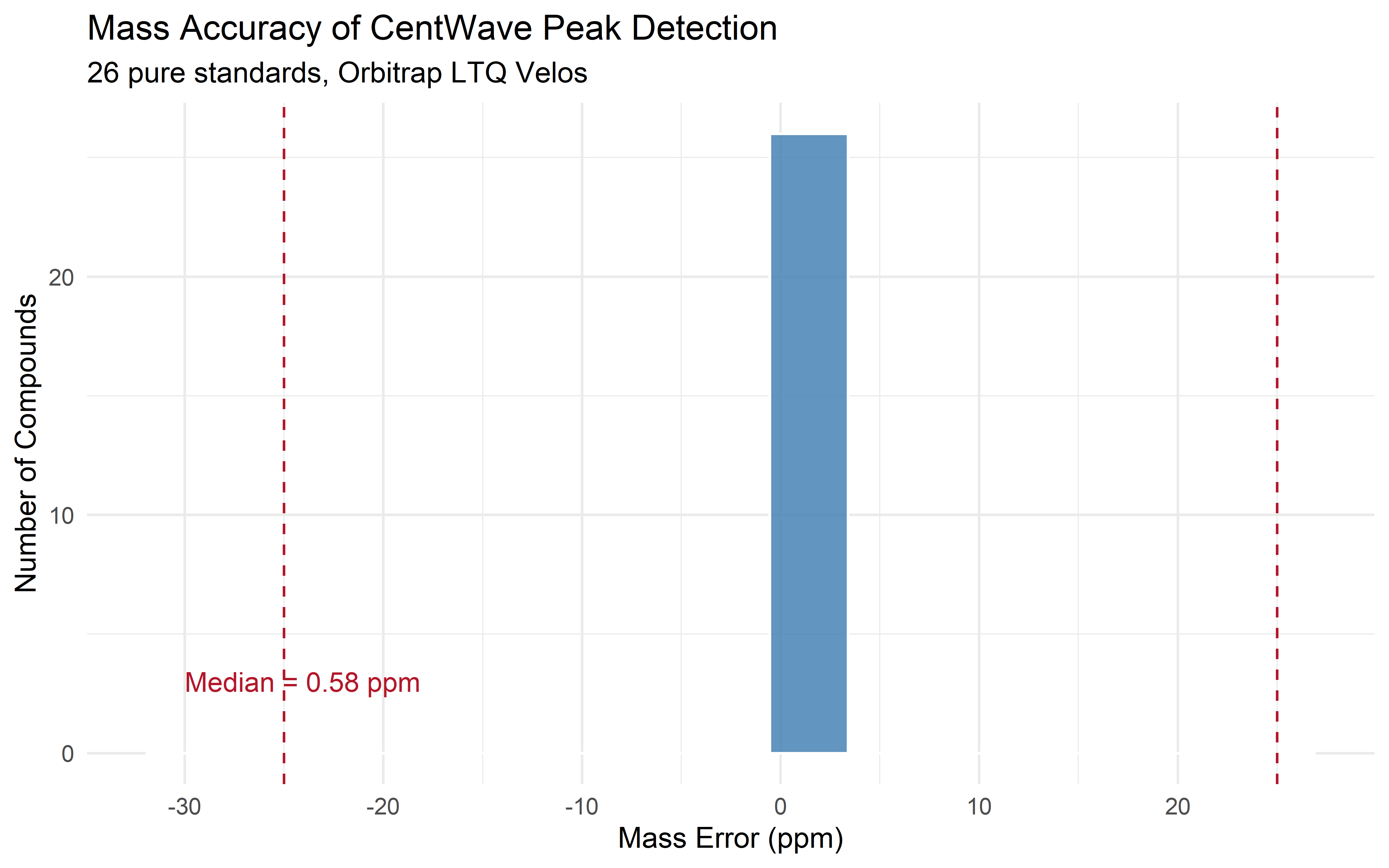
We repeated this analysis on all 26 MTBLS38 standards with known monoisotopic masses. The results validate CentWave on an Orbitrap platform. The pre-computed figure below shows the mass accuracy distribution:
```{r}
#| eval: true
#| echo: true
#| fig-width: 8
#| fig-height: 5
#| label: fig-mass-accuracy-code
#| fig-cap: "Mass accuracy of CentWave-detected peaks vs. known monoisotopic masses across 26 pure metabolite standards."
# Load the pre-computed validation table
peak_val <- read.csv("data/mtbls38/peak_validation.csv")

ggplot(peak_val, aes(x = ppm_error)) +
  geom_histogram(fill = "steelblue", bins = 15, alpha = 0.85,
                 colour = "white") +
  geom_vline(xintercept = c(-25, 25), linetype = "dashed", colour = "#B2182B") +
  annotate("text", x = -30, y = 3,
    label = sprintf("Median = %.2f ppm", median(peak_val$ppm_error)),
    hjust = 0, size = 4, colour = "#B2182B") +
  labs(
    title    = "Mass Accuracy of CentWave Peak Detection",
    subtitle = paste(nrow(peak_val), "pure standards, Orbitrap LTQ Velos"),
    x        = "Mass Error (ppm)",
    y        = "Number of Compounds") +
  theme_minimal(base_size = 12)
```
{#fig-mass-accuracy width=70%}
| Metric | Value |
|--------|-------|
| Standards tested | 26 |
| Detection rate | **100 %** (26 / 26) |
| Median mass error | **0.57 ppm** |
| Best accuracy | glycine betaine: 0.002 ppm |
| Range | 0.001–2.52 ppm — all within ±3 ppm |
::: {.callout-important appearance="simple"}
## Why This Matters
1. **CentWave works.** All 26 known compounds were detected at the expected mass with sub-ppm accuracy. If CentWave cannot find your compound of interest in a biological sample, the issue is likely concentration or matrix suppression — not the peak detection algorithm.
2. **Mass accuracy is not the same as identification.** A 0.57 ppm match tells you the *elemental composition* is consistent, but it does not distinguish isomers (e.g., glucose vs. galactose, both C₆H₁₂O₆ at m/z 179.0556). Chapters 10–11 address how to combine retention time, MS/MS spectra, and isotopic patterns for confident identification.
3. **Parameter tuning matters.** The 26 standards span a wide chromatographic range (RT 7–597 s) and a wide concentration range (intensity 1.3 × 10⁴–5.7 × 10⁷). A single `peakwidth` and `noise` setting correctly detected all of them, demonstrating that CentWave's default parameters are robust for Orbitrap data.
:::
### Effect of SNR Threshold
The `snthresh` parameter is the most impactful tuning knob in CentWave. Setting it too low produces many false-positive peaks; setting it too high misses low-abundance compounds. Using the biotin standard, we tested SNR thresholds from 5 to 100:
```{r}
#| eval: false
#| echo: true
#| fig-width: 8
#| fig-height: 5
snr_values <- c(5, 10, 20, 50, 100)
snr_counts <- sapply(snr_values, function(s) {
  p <- CentWaveParam(ppm = 25, peakwidth = c(5, 60),
                     snthresh = s, noise = 1000, prefilter = c(3, 100))
  nrow(chromPeaks(findChromPeaks(chr, param = p)))
})

snr_df <- data.frame(SNR = factor(snr_values), Peaks = snr_counts)

ggplot(snr_df, aes(x = SNR, y = Peaks)) +
  geom_col(fill = "steelblue", alpha = 0.85) +
  geom_text(aes(label = Peaks), vjust = -0.5, size = 4.5) +
  labs(
    title = "Effect of SNR Threshold — Biotin Standard",
    subtitle = "snthresh = 10 is the sweet spot for Orbitrap data",
    x = "snthresh",
    y = "Peaks Detected") +
  theme_minimal(base_size = 12)
```
At `snthresh = 5`, CentWave reports 13 peaks (many noise-derived). At `snthresh = 10`, it reports 13 peaks as well — but with a cleaner baseline. At `snthresh = 50`, only 8 peaks remain, and at `snthresh = 100`, only 4. **The recommended starting value for Orbitrap data is `snthresh = 10`**, accepting 1–20 peaks per compound and filtering further by mass accuracy and retention time consistency in downstream steps.
::: {.callout-note appearance="simple"}
## Exercise: Validate With Your Own Data
If you have access to internal standards or a standard mixture, run the workflow above on your own mzML files:
1. Look up the exact monoisotopic mass of your standard from [PubChem](https://pubchem.ncbi.nlm.nih.gov/) or [ChEBI](https://www.ebi.ac.uk/chebi/).
2. Extract the EIC within ±25 ppm using `chromatogram(raw, mz = ...)`.
3. Run `findChromPeaks()` with `CentWaveParam` and compare the detected `mz` to the known mass.
4. Compute the mass error in ppm: `abs(mz_found - mz_expected) / mz_expected * 1e6`.
5. If the error exceeds 5 ppm, check your instrument's mass calibration.
This single test can diagnose instrument performance, parameter settings, and software bugs before you invest hours in processing a full batch.
:::
------------------------------------------------------------------------
## Step 2 — Retention Time Alignment
Even identical instrument settings produce small RT drifts between injections due to column aging, temperature fluctuations, and solvent equilibration. Alignment corrects these systematic shifts before peaks are grouped across samples.
`xcms` provides two alignment algorithms:
| Method | Use case |
|----|----|
| `ObiwarpParam` | Global warping; robust when drift is large or samples differ broadly |
| `PeakGroupsParam` | Loess-based correction using shared landmark peaks; fast and interpretable when runs are already close |
```{r}
#| eval: false
xset <- adjustRtime(xset, param = ObiwarpParam(binSize = 0.6))
```
### Checking alignment quality
```{r}
#| eval: false
# Overlay adjusted vs. raw retention times; tight curves indicate good alignment
plotAdjustedRtime(xset)
```
If adjustment produces sharp, noisy deviations, reduce `binSize`. If large drift remains, increase it or switch to Obiwarp with a smaller `gapInit` penalty.
------------------------------------------------------------------------
## Step 3 — Feature Correspondence
Peak grouping answers the question: *which peaks in different samples correspond to the same compound?* `groupChromPeaks()` with `PeakDensityParam` groups peaks that fall within a shared *m/z* and RT window across samples, assigning each group a **feature ID**.
```{r}
#| eval: false
pdp <- PeakDensityParam(
  sampleGroups = sample_meta$condition,
  bw           = 30,      # RT bandwidth for density estimation (seconds)
  minFraction  = 0.5,     # Feature must appear in ≥50 % of samples in at least one group
  minSamples   = 1,
  binSize      = 0.025    # m/z bin size (Daltons)
)

xset <- groupChromPeaks(xset, param = pdp)
```
`minFraction` is the most important tuning parameter here: too low and noise peaks form spurious features; too high and genuine low-abundance compounds are discarded.
```{r}
#| eval: false
# Feature summary
feat_def <- featureDefinitions(xset)
nrow(feat_def)
head(feat_def[, c("mzmed", "rtmed", "npeaks")])
```
------------------------------------------------------------------------
## Step 4 — Fill Missing Peak Areas
After grouping, many features have `NA` in samples where CentWave did not detect a peak. Some are genuine absences; others are real signals that fell just below the detection threshold. `fillChromPeaks()` re-integrates the signal in the expected *m/z*–RT window for every such sample.
```{r}
#| eval: false
xset <- fillChromPeaks(xset, param = ChromPeakAreaParam())
```
> **Caution**: `fillChromPeaks()` will integrate noise if the compound is truly absent. Features where the majority of samples required filling warrant lower confidence in downstream analyses and should be flagged accordingly.
------------------------------------------------------------------------
## Step 5 — Extract the Feature Matrix
```{r}
#| eval: false
feat_mat <- featureValues(xset, value = "into", method = "sum")
dim(feat_mat)   # features × samples

# Wrap in a SummarizedExperiment for downstream analysis
se <- SummarizedExperiment(
  assays  = list(intensity = feat_mat),
  colData = sample_meta
)
se
```
------------------------------------------------------------------------
## Quality Metrics
### Detection rate per feature
Features detected in fewer than half the samples are often noise-derived. Inspect the distribution before carrying them into statistical models:
```{r}
#| eval: false
detection_rate <- rowMeans(!is.na(feat_mat))

data.frame(detection_rate) |>
  ggplot(aes(detection_rate)) +
  geom_histogram(bins = 20, fill = "#4472C4", colour = "white") +
  labs(x = "Fraction of samples with detected signal",
       y = "Number of features",
       title = "Feature detection rate") +
  theme_minimal()
```
### Coefficient of variation in QC pools
If pooled QC samples were injected, compute the per-feature CV to assess technical reproducibility:
```{r}
#| eval: false
qc_idx <- which(colData(se)$condition == "QC")
if (length(qc_idx) >= 2) {
  cv_qc <- apply(
    assay(se)[, qc_idx], 1,
    function(x) sd(x, na.rm = TRUE) / mean(x, na.rm = TRUE) * 100
  )
  message("Median CV in QC samples: ", round(median(cv_qc, na.rm = TRUE), 1), " %")
}
```
A median CV below 30 % indicates acceptable technical reproducibility for untargeted profiling.
------------------------------------------------------------------------
## Summary
| Step | `xcms` function | Key parameter to tune |
|----|----|----|
| Peak detection | `findChromPeaks(CentWaveParam())` | `ppm`, `peakwidth` |
| RT alignment | `adjustRtime(ObiwarpParam())` | `binSize` |
| Feature grouping | `groupChromPeaks(PeakDensityParam())` | `minFraction`, `bw` |
| Peak filling | `fillChromPeaks(ChromPeakAreaParam())` | — |
| Feature matrix export | `featureValues(value = "into")` | `method` |
The `SummarizedExperiment` produced at the end of this chapter is the input for the identification chapters that follow (Chapters 8–11) and for the quantification and statistical workflows in Parts III–V.
## Exercises
1. **Parameter Exploration**: Run `findChromPeaks()` on the `faahKO` dataset with `ppm = c(10, 20, 40)`. Plot the number of detected features against `ppm`. At what point do diminishing returns set in?
2. **Alignment Diagnosis**: Before and after `adjustRtime()`, extract the retention times of a known internal standard peak. Compute the CV of its RT across all runs. Did alignment improve the CV?
3. **Grouping Sensitivity**: Vary `minFraction` from 0.3 to 0.9 in steps of 0.1 and report how the number of consensus features changes. Propose a defensible `minFraction` for a study with 12 samples per group and explain your choice.
4. **Gap-Filling Impact**: Compare the percentage of missing values in your feature matrix before and after `fillChromPeaks()`. In which types of features (abundant vs. low-intensity) does gap filling recover the most values?
------------------------------------------------------------------------
## Further Reading
- Smith CA, Want EJ, O'Maille G, Abagyan R, Siuzdak G. XCMS: processing mass spectrometry data for metabolite profiling using nonlinear peak alignment, matching, and identification. *Analytical Chemistry*. 2006;78(3):779–787.
- Benton HP, Want EJ, Ebbels TMD. Correction of mass calibration gaps in liquid chromatography–mass spectrometry metabolomics data. *Bioinformatics*. 2010;26(19):2488–2489.
- Rainer J, Vicini A, Salzer L, et al. A modular and expandable ecosystem for metabolomics data annotation in R. *Metabolites*. 2022;12(2):173.
- xcms package documentation: <https://bioconductor.org/packages/xcms>
## Session Information
```{r}
sessionInfo()
```