17  Normalize Across Samples and Batches

“Before you ask which proteins or metabolites changed, you need to ask whether the matrix is trustworthy.”

Load the same pooled sample twice and you will get two different numbers. Run a study across two weeks, two columns, or two reagent lots, and that technical variation can swamp the biology you came to measure — or, worse, mimic it. Normalization and batch correction are how you make samples comparable without scrubbing away the signal. Do too little and batch effects masquerade as discoveries; do too much and you erase the differences that are real.

WarningThe One Mistake to Avoid

Correcting for batch twice — once with ComBat and again as a model covariate. Removing the effect twice biases your inference. Correct for visualization, or model the covariate for testing; never both.

17.1 Learning Objectives

By the end of this chapter you will be able to:

• Log‑transform and scale feature matrices correctly
• Apply common normalization methods: median, quantile, LOESS, and TIC‑based
• Diagnose and correct batch effects using ComBat
• Compare normalization methods using CV and PCA
• Produce an analysis‑ready intensity matrix with appropriate QC visualisations

17.2 Why Normalization Is Critical for MS Data

Raw MS feature tables contain systematic non‑biological variation:

Source	Example	Consequence
Sample loading	Different protein/metabolite amounts injected	Global intensity shifts
Instrument sensitivity	Detector aging over time	Drift across injection order
Batch effects	Different columns, reagent lots, operators	Discontinuous jumps
Run‑to‑run variation	Mobile phase, temperature, flow rate	Unpredictable changes

Normalization does not remove all unwanted variation – that requires careful experimental design and batch correction. But it is the essential first step to make samples comparable.

17.2.1 Choosing a Normalization Method

The choice of normalization method depends on the structure of the unwanted variation and the properties of your data. There is no universally “best” method — the choice is a modeling decision, not a default:

Method	Assumption	Best When	Weakness
Median centering	Systematic shift is additive and uniform across features	Small datasets, simple designs	Cannot correct non-linear or feature-dependent bias
Quantile normalisation	Feature intensity distributions are identical across samples (up to shift)	Microarrays; large p with similar distributions	Distorts distributions when they differ fundamentally
Cyclic LOESS	Bias is smooth in intensity space	Dye-bias in two-colour arrays; MS when bias varies with intensity	Computationally expensive for many samples
TIC normalisation	Total ion current is proportional to sample amount	LC-MS with consistent sample composition	Fails when a few highly abundant features dominate TIC
Internal standard (IS)	IS behaves identically to analytes of interest	Targeted MS with stable-isotope IS	Requires IS; IS may degrade or ionise differently
ComBat (batch correction)	Batch effects are additive on the log scale; batches share biological composition	Multi-batch studies with balanced designs	Over-corrects if batches are confounded with biology

17.2.2 The Decision Rule for MS Data

For untargeted LC-MS metabolomics or proteomics, a robust workflow is:

1. Log-transform first — MS intensity data are log-normal; normalisation on the linear scale amplifies high-abundance features
2. Median normalisation as default — robust to outliers, minimal assumptions
3. Assess with PCA before and after — samples should cluster by biology, not batch
4. Apply batch correction (ComBat) only if batch effects persist after median normalisation AND batches are not confounded with biological groups
5. Validate with QC pools — CV in pooled QC samples should decrease after normalisation

Never skip PCA before/after normalisation. If normalisation fails to separate samples by biological group or fails to reduce technical clustering, the downstream analysis will produce artefacts regardless of statistical sophistication.

This chapter assumes you already have a feature table (rows = features, columns = samples) from preprocessing (e.g., xcms or DEP). We will work with a realistic simulated dataset and also show how to adapt to real msdata examples.

---

17.3 Setup and Required Packages

BiocManager::install(c(
  "limma",        # Normalization functions
  "preprocessCore", # Quantile normalization
  "impute",       # k‑NN imputation
  "msdata",
  "ggplot2",
  "dplyr",
  "tidyr"
))

library(limma)
library(preprocessCore)
library(impute)
library(msdata)
library(ggplot2)
library(dplyr)
library(tidyr)

set.seed(42)

---

17.4 Step 1: From Feature Table to Analysis‑Ready Matrix

17.4.1 Simulate a Realistic MS Feature Table

We simulate 150 metabolites and 24 samples (3 batches, 2 groups). True biological signal exists for the first 30 metabolites.

n_metabolites <- 150
n_samples <- 24
n_batches <- 3
samples_per_batch <- n_samples / n_batches

# Sample metadata
metadata <- data.frame(
  sample_id = paste0("S", 1:n_samples),
  batch = rep(paste0("Batch", 1:n_batches), each = samples_per_batch),
  condition = rep(rep(c("Control", "Treatment"), each = samples_per_batch/2), times = n_batches),
  injection_order = 1:n_samples
)

# Base intensities (log‑normal)
intensity_raw <- matrix(rlnorm(n_metabolites * n_samples, meanlog = 10, sdlog = 1.5),
                        nrow = n_metabolites, ncol = n_samples)
rownames(intensity_raw) <- paste0("Metab_", 1:n_metabolites)
colnames(intensity_raw) <- metadata$sample_id

# Add batch effect: Batch2 has +30% intensity, Batch3 has -20%
batch_effect <- c(0, 0.3, -0.2)
for (i in 1:n_batches) {
  idx <- metadata$batch == paste0("Batch", i)
  intensity_raw[, idx] <- intensity_raw[, idx] * (1 + batch_effect[i])
}

# Add treatment effect for first 30 metabolites (2‑fold up in Treatment)
treatment_idx <- metadata$condition == "Treatment"
intensity_raw[1:30, treatment_idx] <- intensity_raw[1:30, treatment_idx] * 2

# Add missing values (20% random, plus 10% MNAR in treatment group)
set.seed(42)
na_random <- matrix(runif(n_metabolites * n_samples) < 0.2, nrow = n_metabolites, ncol = n_samples)
na_mnar <- matrix(FALSE, nrow = n_metabolites, ncol = n_samples)
# MNAR: low‑intensity features in treatment group
low_intensity <- intensity_raw < median(intensity_raw)
na_mnar[1:30, treatment_idx] <- low_intensity[1:30, treatment_idx] & runif(30 * sum(treatment_idx)) < 0.5
intensity_raw[na_random | na_mnar] <- NA

cat(sprintf("Feature table: %d metabolites × %d samples\n", n_metabolites, n_samples))

Feature table: 150 metabolites × 24 samples

cat(sprintf("Overall missing rate: %.1f%%\n", 100 * mean(is.na(intensity_raw))))

Overall missing rate: 22.8%

17.4.2 Log Transformation

MS intensities are heteroscedastic – variance increases with mean. Log2 transformation stabilises variance and makes multiplicative effects additive.

# Log2 transform (add 1 to avoid log(0) if zeros present)
intensity_log <- log2(intensity_raw + 1)

# Compare distribution before/after
plot_df <- data.frame(
  raw = intensity_raw[!is.na(intensity_raw)],
  log = intensity_log[!is.na(intensity_log)]
)
plot_df |>
  pivot_longer(everything(), names_to = "transform", values_to = "intensity") |>
  ggplot(aes(x = intensity, fill = transform)) +
  geom_density(alpha = 0.5) +
  facet_wrap(~transform, scales = "free") +
  labs(title = "Raw vs log2‑transformed intensities") +
  theme_minimal()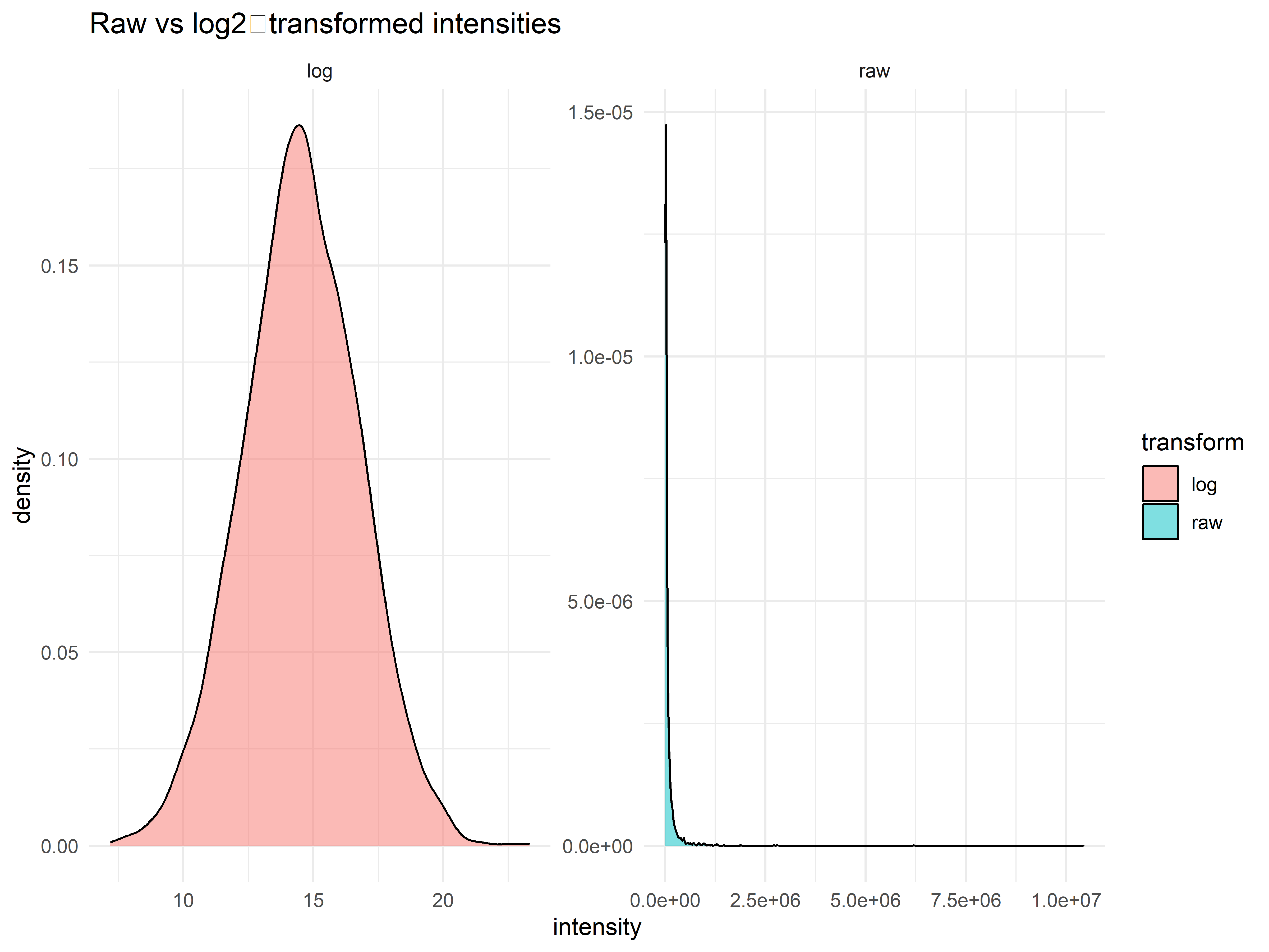

---

17.5 Step 2: Scaling and Centering

After log transformation, we often center and scale to give each feature equal influence in multivariate analysis.

• Centering: subtract mean → features have mean zero
  
• Scaling: divide by standard deviation → features have unit variance

# Center and scale (robust: use median and MAD)
center_scale <- function(mat, robust = TRUE) {
  if (robust) {
    center <- apply(mat, 1, median, na.rm = TRUE)
    scale <- apply(mat, 1, mad, na.rm = TRUE)
    scale[scale == 0] <- 1
  } else {
    center <- rowMeans(mat, na.rm = TRUE)
    scale <- apply(mat, 1, sd, na.rm = TRUE)
    scale[scale == 0] <- 1
  }
  scaled <- (mat - center) / scale
  return(scaled)
}

intensity_scaled <- center_scale(intensity_log, robust = TRUE)

# Check one metabolite
meta_id <- rownames(intensity_scaled)[1]
data.frame(
  original = intensity_log[meta_id, ],
  scaled = intensity_scaled[meta_id, ]
) |>
  pivot_longer(everything()) |>
  ggplot(aes(x = value)) + geom_histogram(bins = 20) + facet_wrap(~name, scales = "free")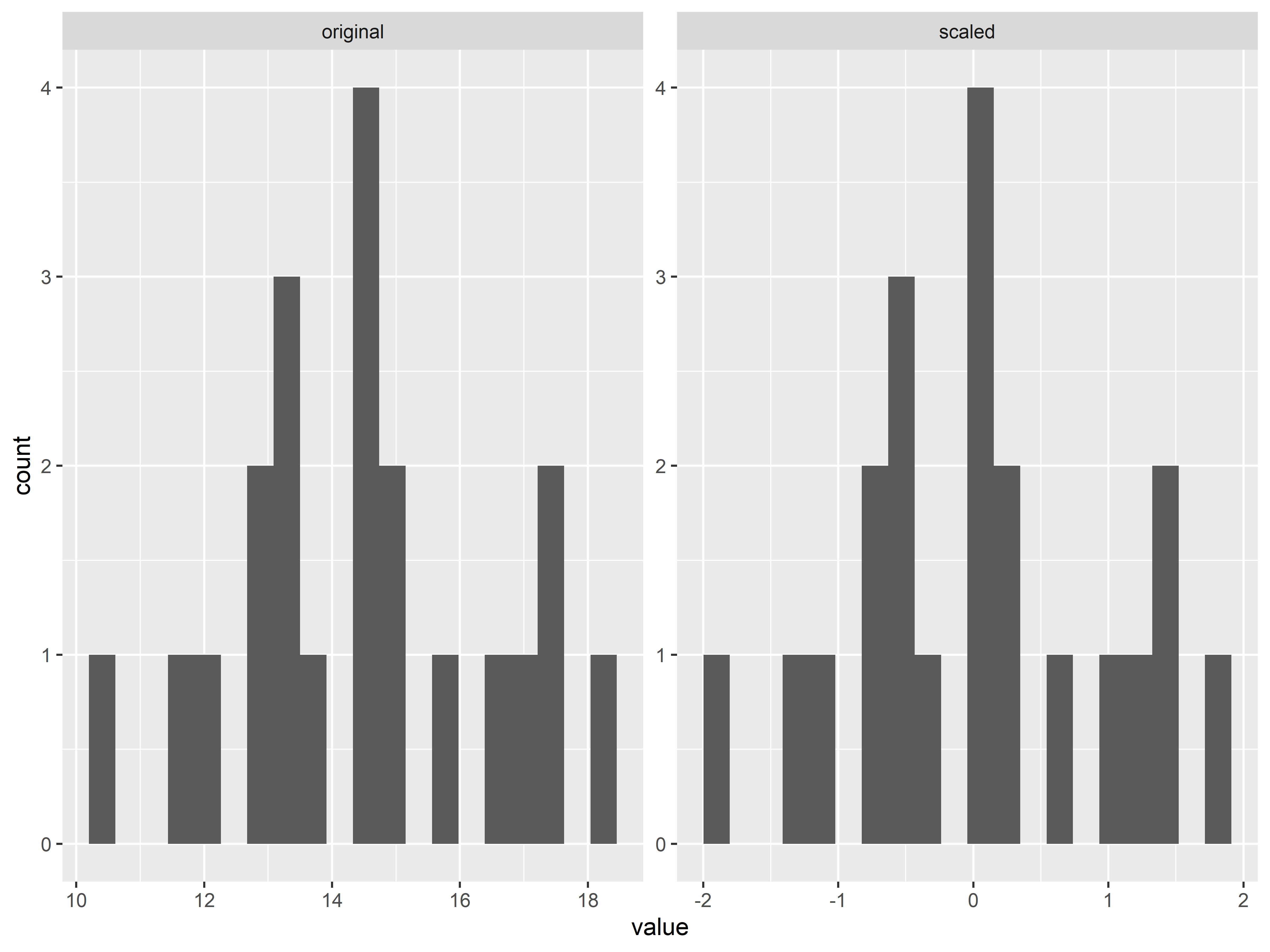

When to use scaling?
- PCA, heatmaps, clustering: yes – prevents high‑abundance features dominating
- Univariate testing (t‑test, limma): usually not necessary because each feature is tested independently

---

17.6 Step 3: Normalization Methods

Normalization adjusts for sample‑wide intensity differences. Always normalise after log transform unless using TIC‑based (which works on raw scale).

17.6.1 Method 1: Median Normalization

Assume most features do not change between samples – scale each sample to have the same median intensity.

median_norm <- function(mat) {
  sample_medians <- apply(mat, 2, median, na.rm = TRUE)
  global_median <- median(sample_medians, na.rm = TRUE)
  norm_mat <- sweep(mat, 2, sample_medians / global_median, FUN = "/")
  return(norm_mat)
}

intensity_med_norm <- median_norm(intensity_log)

17.6.2 Method 2: TIC (Total Ion Current) Normalization

Scale each sample by its total sum of intensities. Works on raw or log scale (but log then TIC is unusual). Best on raw scale.

tic_norm <- function(mat) {
  # mat is raw intensities (not log)
  sample_sums <- colSums(mat, na.rm = TRUE)
  global_mean <- mean(sample_sums, na.rm = TRUE)
  norm_mat <- sweep(mat, 2, sample_sums / global_mean, FUN = "/")
  return(norm_mat)
}

# Apply to raw intensities (with NA handling)
intensity_raw_imp <- intensity_raw
intensity_raw_imp[is.na(intensity_raw_imp)] <- 0  # temporary for TIC only
intensity_tic_norm <- tic_norm(intensity_raw_imp)
# Then log transform
intensity_tic_norm_log <- log2(intensity_tic_norm + 1)

17.6.3 Method 3: Quantile Normalization

Forces all samples to have the same intensity distribution. Assumes that the overall distribution of features is identical across samples – often too strong for MS data, but can be useful for removing batch effects.

# Requires complete data – impute first (simple column median)
intensity_imp <- intensity_log
for (j in 1:ncol(intensity_imp)) {
  intensity_imp[is.na(intensity_imp[, j]), j] <- median(intensity_imp[, j], na.rm = TRUE)
}
intensity_quantile <- normalize.quantiles(intensity_imp)
colnames(intensity_quantile) <- colnames(intensity_imp)
rownames(intensity_quantile) <- rownames(intensity_imp)

# Compare original vs quantile
plot_df <- data.frame(
  original = intensity_log[, 1],
  quantile = intensity_quantile[, 1]
)
ggplot(plot_df, aes(x = original, y = quantile)) + geom_point(alpha = 0.5) +
  geom_abline(slope = 1, intercept = 0, color = "red") +
  labs(title = "Quantile normalization effect (Sample 1)")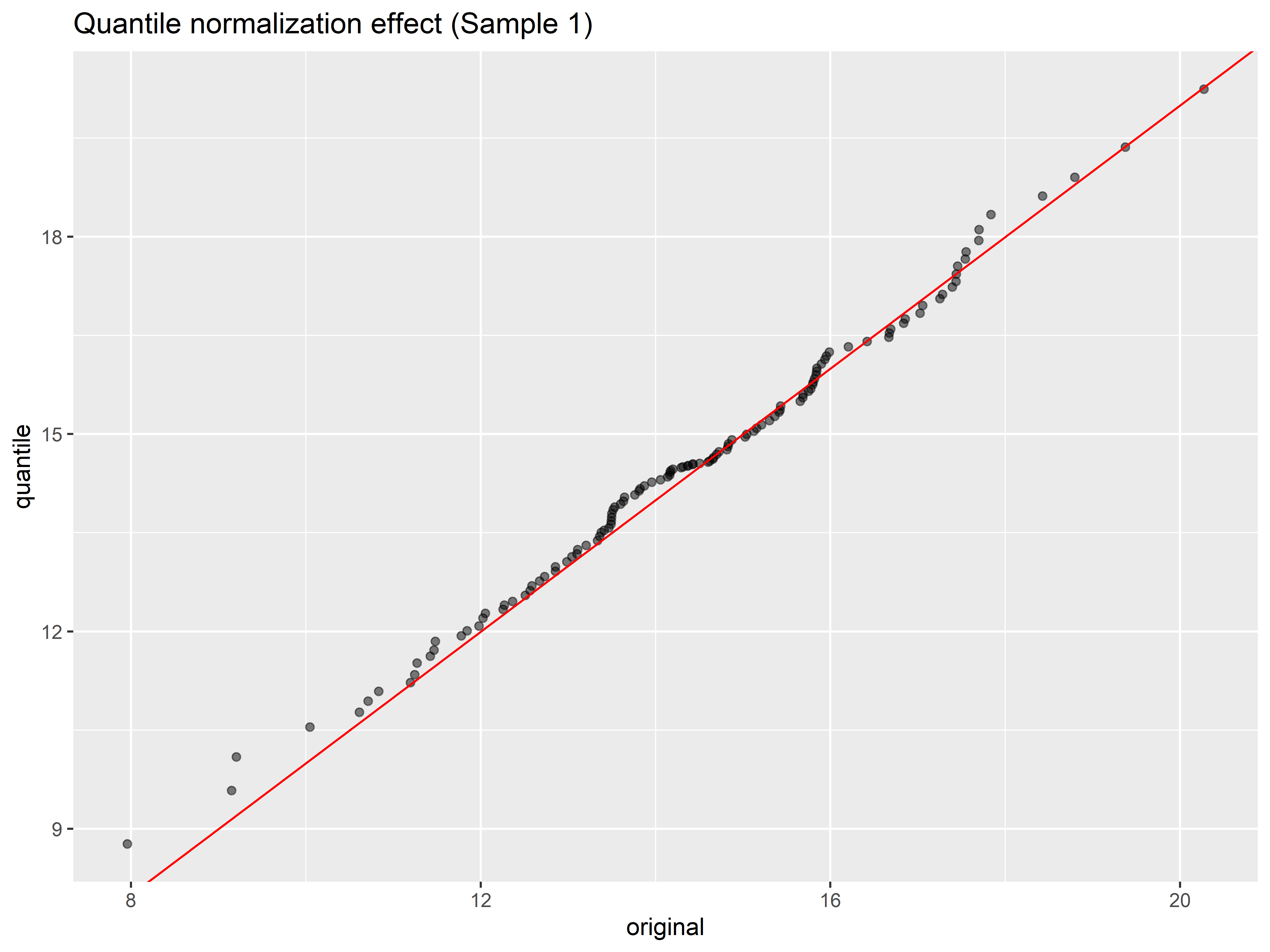

17.6.4 Method 4: LOESS Normalization (for injection order drift)

If intensity drifts systematically with injection order, LOESS smoothing can correct it.

loess_norm <- function(mat, injection_order) {
  # mat: log‑transformed, rows = features, cols = samples
  norm_mat <- mat
  for (i in 1:nrow(mat)) {
    y <- mat[i, ]
    if (sum(!is.na(y)) > 5) {
      loess_fit <- loess(y ~ injection_order, span = 0.75)
      pred <- predict(loess_fit)
      norm_mat[i, ] <- y - pred + mean(y, na.rm = TRUE)
    }
  }
  return(norm_mat)
}

# Apply (requires injection order in metadata)
injection_order <- metadata$injection_order
intensity_loess_norm <- loess_norm(intensity_log, injection_order)

17.6.5 Compare Normalization Methods

# Function to compute median CV per sample (after log)
calc_sample_cv <- function(mat) {
  apply(mat, 2, function(x) sd(x, na.rm = TRUE) / mean(x, na.rm = TRUE))
}

cv_df <- data.frame(
  raw = calc_sample_cv(intensity_log),
  median = calc_sample_cv(intensity_med_norm),
  quantile = calc_sample_cv(intensity_quantile),
  tic = calc_sample_cv(intensity_tic_norm_log)
)

cv_df |>
  pivot_longer(everything(), names_to = "method", values_to = "cv") |>
  ggplot(aes(x = method, y = cv)) + geom_boxplot() +
  labs(title = "Sample CV by normalization method", y = "CV (coefficient of variation)")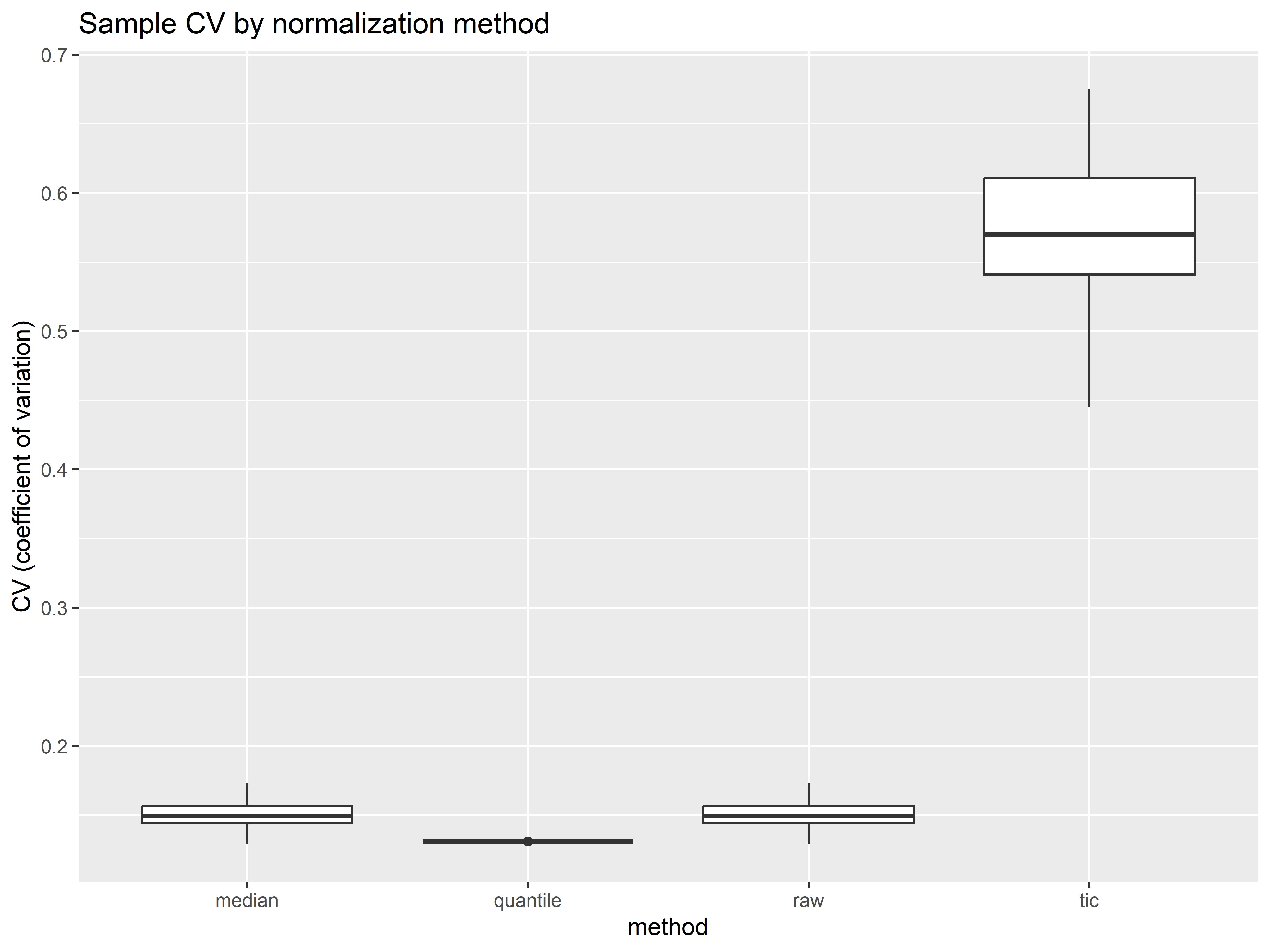

Interpretation: Lower median CV indicates better removal of sample‑wide variation. Quantile often gives lowest CV but may over‑correct.

---

17.7 Common Pitfalls and Solutions

Pitfall	Consequence	Solution
Normalising before log transform	Multiplicative effects not stabilised	Always log‑transform first (except TIC)
Using quantile normalisation on MS data	Removes true biological variation	Use median or LOESS; quantile only for strong batch effects
Applying ComBat before splitting train/test	Test leaks into batch model	Correct batches inside cross‑validation or on training data only
Scaling before univariate testing	Inflates or deflates effect sizes	Scale only for multivariate methods (PCA, heatmaps)
Skipping PCA check after normalization	Residual batch structure invisible	Always plot PCA coloured by batch before proceeding

---

17.8 Exercises

17.8.1 Exercise 1: Compare Normalization Methods

Using the simulated dataset, apply median, quantile, TIC, and LOESS normalization. Which gives the lowest variance within batches? Use boxplots of sample CV.

# Your code here

17.8.2 Exercise 2: Batch Effect Severity

Simulate a stronger batch effect (larger batch_shift). At what point does median normalization fail? Does ComBat still correct adequately? Use PCA before/after to compare.

# Your code here

17.8.3 Exercise 3: LOESS Normalization

Replace median normalization with limma::normalizeCyclicLoess(). Compare the sample-to-sample correlation matrices before and after normalization using pheatmap.

# Your code here

17.8.4 Exercise 4: Full Normalization Pipeline

Write a function that takes a raw feature table and metadata and applies log transform → median normalization → ComBat batch correction. Return the corrected matrix and a PCA plot. Run it on the simulated data.

# Your code here

---

17.9 Summary

17.9.1 Key Steps in Order

Step	Purpose	R Code (example)
Log transform	Stabilise variance	log2(x + 1)
Normalize	Remove sample‑wide bias	median_norm(), normalize.quantiles()
Check PCA	Detect residual batch structure	prcomp() + ggplot2
Batch correction	Remove technical batch effects	sva::ComBat()
(Optional) Scale	Equalise feature variance for multivariate	scale() with robust options

17.9.2 Recommended Default Workflow for MS Data

1. Log2 transform
2. Normalize: median or TIC (check which reduces CV best)
3. Inspect PCA coloured by batch — if clusters visible, proceed to step 4
4. ComBat batch correction (parametric for large batches, non‑parametric for small)
5. Scale only for multivariate analysis (PCA, heatmaps, clustering)
6. Missing values → handled in the next chapter

17.9.3 Resources

• limma normalization functions
• preprocessCore quantile normalization
• sva/ComBat batch correction

---

17.10 Session Information

sessionInfo()

R version 4.5.1 (2025-06-13 ucrt)
Platform: x86_64-w64-mingw32/x64
Running under: Windows 11 x64 (build 26200)

Matrix products: default
  LAPACK version 3.12.1

locale:
[1] LC_COLLATE=English_Switzerland.utf8  LC_CTYPE=English_Switzerland.utf8   
[3] LC_MONETARY=English_Switzerland.utf8 LC_NUMERIC=C                        
[5] LC_TIME=English_Switzerland.utf8    

time zone: Europe/Zurich
tzcode source: internal

attached base packages:
[1] stats     graphics  grDevices utils     datasets  methods   base     

other attached packages:
[1] tidyr_1.3.2           dplyr_1.2.1           ggplot2_4.0.3        
[4] msdata_0.48.0         impute_1.82.0         preprocessCore_1.70.0
[7] limma_3.64.3         

loaded via a namespace (and not attached):
 [1] gtable_0.3.6       jsonlite_2.0.0     compiler_4.5.1     tidyselect_1.2.1  
 [5] scales_1.4.0       yaml_2.3.12        fastmap_1.2.0      statmod_1.5.2     
 [9] R6_2.6.1           labeling_0.4.3     generics_0.1.4     knitr_1.51        
[13] htmlwidgets_1.6.4  tibble_3.3.1       pillar_1.11.1      RColorBrewer_1.1-3
[17] rlang_1.3.0        xfun_0.60          S7_0.2.2           otel_0.2.0        
[21] cli_3.6.5          withr_3.0.3        magrittr_2.0.5     digest_0.6.37     
[25] grid_4.5.1         lifecycle_1.0.5    vctrs_0.7.3        evaluate_1.0.5    
[29] glue_1.8.1         farver_2.1.2       rmarkdown_2.31     purrr_1.2.2       
[33] tools_4.5.1        pkgconfig_2.0.3    htmltools_0.5.9