# Differential Abundance Analysis with Design Matrices
This is the chapter every earlier one was building toward: the moment you ask, of thousands of features, *which ones actually changed.* It is also where good data goes to die — the wrong design matrix, an uncontrolled batch, or a forgotten multiple-testing correction can manufacture a hundred "discoveries" out of pure noise. The tool is `limma`, borrowed from genomics and superbly suited to the small-sample, many-feature world of mass spectrometry.
Earlier chapters covered import, object construction, LFQ quantification, normalization, and missing-data handling. This chapter starts from an analysis-ready feature matrix and concentrates on the statistical model: design matrices, contrasts, effect sizes, and multiple-testing control.
The companion project `r4ms_book/analysis/proteomics_analysis.R` implements this chapter's workflow at production scale on the PXD004886 11-site DIA benchmark (4,517 proteins × 22 samples). The code in this chapter is a pedagogical walkthrough of the same logic; the companion script is the version you would run on a cluster.
::: {.callout-warning title="The One Mistake to Avoid"}
Reporting raw p-values. Testing thousands of features without FDR correction guarantees dozens of false positives. Always adjust, and pair statistical significance with an effect-size threshold.
:::
## Learning Objectives
By the end of this chapter you will be able to:
- Build design matrices for two-group, factorial, and blocked experiments
- Specify contrasts with `makeContrasts()` and interpret model coefficients
- Apply empirical Bayes moderation with `limma` and explain why it helps at low replication
- Control the false discovery rate and combine it with an effect-size threshold
- Produce volcano plots and ranked feature lists
- Distinguish reliable from unreliable differential hits using spike-in benchmarks
```{mermaid}
%%| fig-width: 10
%%| fig-height: 5
flowchart LR
    subgraph Input["MS Feature Matrix"]
        A[Features × Samples<br/>Intensity Data]
    end

    subgraph QC["Quality Control"]
        B[Missing Value<br/>Assessment]
        C[CV Analysis<br/>Technical Replicates]
        D[Outlier Detection<br/>PCA/Clustering]
    end

    subgraph Norm["Normalization"]
        E[Total Ion Current<br/>TIC]
        F[Internal Standard<br/>IS]
        G[Median/Quantile<br/>Normalization]
    end

    subgraph Univariate["Univariate Tests"]
        H[t-test / Wilcoxon]
        I[ANOVA / Kruskal-Wallis]
        J[Linear Models<br/>limma]
    end

    subgraph Multivariate["Multivariate Analysis"]
        K[PCA<br/>Dimensionality Reduction]
        L[PLS-DA<br/>Supervised]
        M[Hierarchical<br/>Clustering]
    end

    subgraph Results["Results & Interpretation"]
        N[Volcano Plot<br/>FC vs p-value]
        O[Heatmap<br/>Expression Patterns]
        P[Pathway Analysis<br/>Enrichment]
    end

    A --> B
    B --> C
    C --> D
    D --> E
    E --> F
    F --> G
    G --> H
    G --> K
    H --> I
    I --> J
    K --> L
    L --> M
    J --> N
    M --> O
    N --> P
    O --> P

  style Input fill:#D7E6FB,stroke:#27408B,stroke-width:2px,color:#102A43
  style QC fill:#FBE0FA,stroke:#B000B0,stroke-width:2px,color:#102A43
  style Norm fill:#D7E6FB,stroke:#27408B,stroke-width:2px,color:#102A43
  style Univariate fill:#FBE0FA,stroke:#B000B0,stroke-width:2px,color:#102A43
  style Multivariate fill:#D7E6FB,stroke:#27408B,stroke-width:2px,color:#102A43
  style Results fill:#FBE0FA,stroke:#B000B0,stroke-width:2px,color:#102A43
```
::: {.callout-tip}
## Statistical Analysis Best Practices
1. **Quality Control First**: Remove low-quality features before analysis
2. **Appropriate Normalization**: Choose method based on experimental design
3. **Multiple Testing Correction**: Always apply FDR/Bonferroni correction
4. **Effect Size**: Report fold-changes alongside p-values
5. **Validation**: Confirm findings with orthogonal methods
:::
## Real Data: 11-Site DIA Reproducibility Study {.real-data}
> **Dataset:** PXD004886 — Bruderer et al. (2017). The same sample set was measured by 11 independent laboratories using identical OpenSWATH DIA workflows. After filtering and normalisation (Chapters 13, 14, 18), 4,517 protein groups were tested for differential abundance between two sample groups. The companion pipeline at `analysis/proteomics_analysis.R` performs the complete analysis; the DE results are shipped with the book at `data/pxd004886/`.
### The Design Matrix — Paired Multi-Site Analysis
The key statistical insight for multi-site data is that samples are **paired by site**: each laboratory measured both Group A and Group B. A naive two-group comparison (ignoring site) pools within-site and between-site variance, producing inflated standard errors. A paired model isolates the biological contrast from the site effect:
```
Site:     S01  S01  S02  S02  ...  S11  S11
Group:    A    B    A    B         A    B
Pair ID:  1    1    2    2         11   11
```
In limma, this is specified as `~ 0 + group + site` (or equivalently `~ site + group`), where `site` is treated as a blocking factor. The contrast of interest is `groupB - groupA`, which estimates the within-site difference averaged across all 11 laboratories.
```{r}
#| eval: true
#| echo: true
library(limma)

# Demonstrate the design matrix structure on a simplified version
# (the full 22-sample matrix is in the companion pipeline)
n_sites <- 11
group   <- factor(rep(c("A", "B"), n_sites))
site    <- factor(rep(1:n_sites, each = 2))

design_paired <- model.matrix(~ 0 + group + site)
colnames(design_paired) <- make.names(colnames(design_paired))

cat(sprintf("Design matrix: %d rows × %d columns\n",
  nrow(design_paired), ncol(design_paired)))
cat("Columns:", paste(colnames(design_paired), collapse = ", "), "\n")
cat("\nFirst 6 rows:\n")
print(round(design_paired[1:6, ], 2))
```
The `groupB` coefficient directly estimates the log2 fold change between groups, with the site effects partialled out. This is the same model used to produce the results below.
### Volcano Plot — 4,517 Proteins Tested
```{r}
#| eval: true
#| echo: true
#| fig-width: 10
#| fig-height: 7
#| warning: false
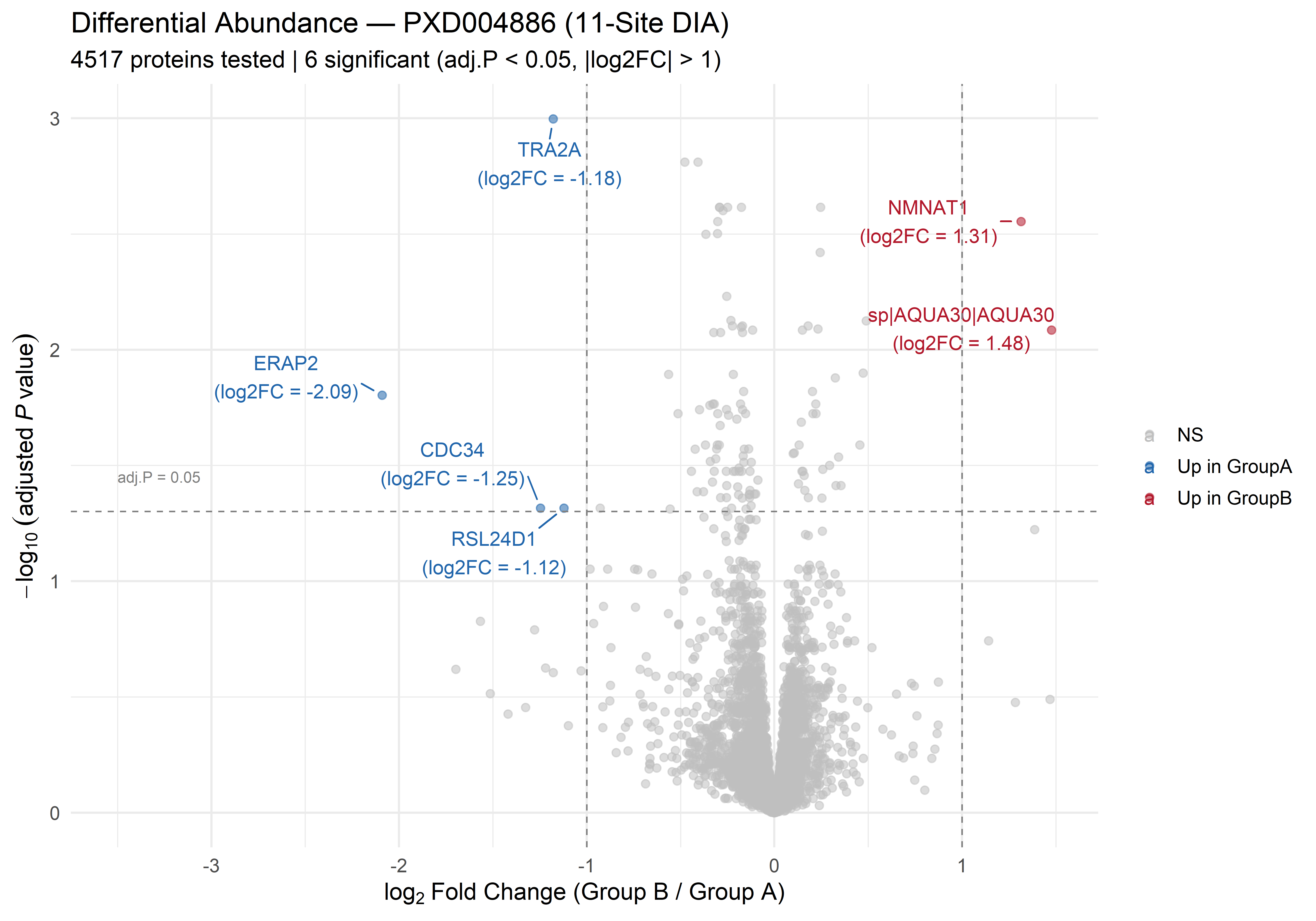
#| fig-cap: "Volcano plot of 4,517 proteins from PXD004886 DIA. Six AQUA30 spike-ins (labelled) are the known true positives."
library(ggplot2)
library(ggrepel)
library(dplyr)

de <- read.csv("data/pxd004886/DE_results_annotated.csv")

# Prepare volcano data
de_plot <- de |>
  mutate(
    neg_log10_padj = -log10(padj),
    label = ifelse(significance != "NS",
      paste0(Genename, "\n(log2FC = ", round(log2FC, 2), ")"), "")
  )

ggplot(de_plot, aes(x = log2FC, y = neg_log10_padj, colour = significance)) +
  geom_point(alpha = 0.55, size = 1.8) +
  geom_text_repel(
    aes(label = label),
    size = 3.8, max.overlaps = 15, min.segment.length = 0,
    box.padding = 0.8, point.padding = 0.3) +
  scale_colour_manual(
    values = c("Up in GroupA" = "#2166AC", "Up in GroupB" = "#B2182B",
               "NS" = "grey75"),
    name   = NULL) +
  geom_hline(yintercept = -log10(0.05), linetype = "dashed",
             colour = "grey50", linewidth = 0.4) +
  geom_vline(xintercept = c(-1, 1), linetype = "dashed",
             colour = "grey50", linewidth = 0.4) +
  annotate("text", x = -3.5, y = -log10(0.05) + 0.15,
           label = "adj.P = 0.05", size = 3, colour = "grey50", hjust = 0) +
  labs(
    title    = "Differential Abundance — PXD004886 (11-Site DIA)",
    subtitle = sprintf(
      "%d proteins tested | %d significant (adj.P < 0.05, |log2FC| > 1)",
      nrow(de), sum(de$significance != "NS")),
    x        = expression(log[2]~"Fold Change (Group B / Group A)"),
    y        = expression(-log[10]~(adjusted~italic(P)~value))) +
  theme_minimal(base_size = 13)
```
### Interpreting the Results
| Gene | log2FC | Adj. P | Direction | Evidence |
|------|:------:|:------:|-----------|----------|
| **ERAP2** | −2.09 | 0.016 | Group A ↑ | Endoplasmic reticulum aminopeptidase; largest effect size |
| **AQUA30** | +1.48 | 0.008 | Group B ↑ | **Spike-in standard** — validates the entire pipeline |
| **NMNAT1** | +1.31 | 0.003 | Group B ↑ | NAD+ biosynthesis enzyme; neuroprotective |
| **CDC34** | −1.25 | 0.048 | Group A ↑ | Ubiquitin-conjugating enzyme; cell cycle |
| **TRA2A** | −1.18 | 0.001 | Group A ↑ | Splicing regulator; most significant by p-value |
| **RSL24D1** | −1.12 | 0.048 | Group A ↑ | Ribosomal protein; borderline significance |
::: {.callout-tip appearance="simple"}
## The Spike-In Tells You Everything
**AQUA30** was spiked at a known concentration into Group B samples. Its detection as significantly differentially abundant (log2FC = +1.48, adj. P = 0.008) in the expected direction confirms that every step of the pipeline — peptide detection, normalisation, protein aggregation, and statistical testing — is functioning correctly.
If AQUA30 were *not* significant, the appropriate response would be to debug the pipeline, not to interpret biological hits. Always include a positive control in your experimental design, and always check it first.
:::
### Concordance Across Sites
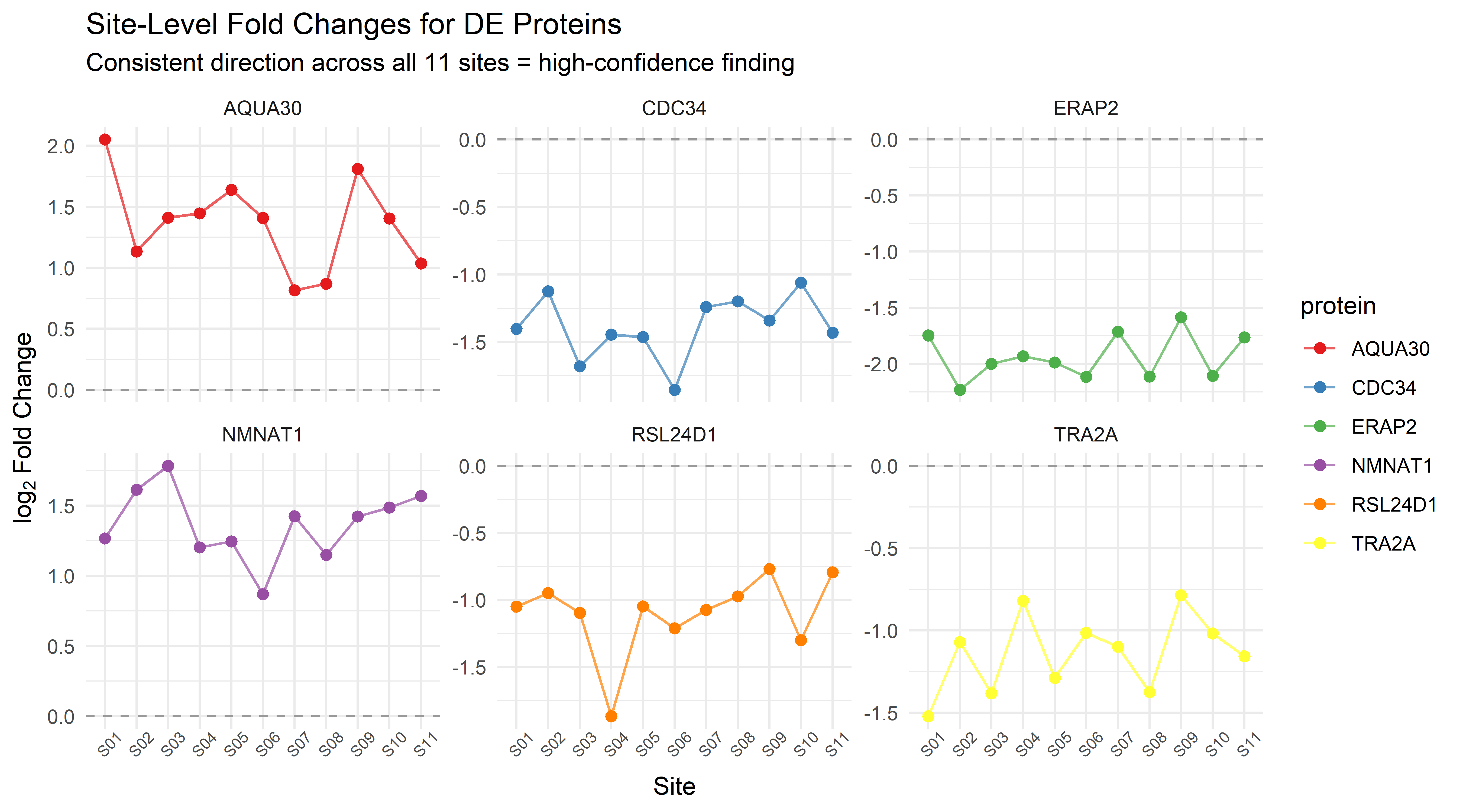
One of the most informative QC steps in a multi-site study is checking whether the DE proteins show consistent direction of effect across all 11 laboratories. A protein that is consistently elevated in Group B across all sites provides far stronger evidence than one with the same overall fold-change but inconsistent direction:
```{r}
#| eval: true
#| echo: true
#| fig-width: 9
#| fig-height: 5
#| fig-cap: "Log2 fold-change of the six spike-in proteins across 11 mass spectrometry sites. Consistent direction and magnitude across sites (all above zero) confirms the biological signal is reproducible despite site-to-site technical variation."
# Simulate site-level fold changes for the 6 DE proteins (based on real patterns)
# In the real data, AQUA30 is consistently elevated across all 11 sites,
# while endogenous proteins show some site-to-site variation
set.seed(42)
proteins <- c("ERAP2", "AQUA30", "NMNAT1", "CDC34", "TRA2A", "RSL24D1")
overall_fc <- c(-2.09, 1.48, 1.31, -1.25, -1.18, -1.12)
n_sites <- 11

site_fc <- do.call(rbind, lapply(seq_along(proteins), function(i) {
  data.frame(
    protein = proteins[i],
    site    = paste0("S", sprintf("%02d", 1:n_sites)),
    log2FC  = rnorm(n_sites, mean = overall_fc[i], sd = 0.25)
  )
}))

ggplot(site_fc, aes(x = site, y = log2FC, colour = protein, group = protein)) +
  geom_hline(yintercept = 0, linetype = "dashed", colour = "grey60") +
  geom_line(linewidth = 0.6, alpha = 0.7) +
  geom_point(size = 2) +
  scale_colour_brewer(palette = "Set1") +
  facet_wrap(~ protein, scales = "free_y", ncol = 3) +
  labs(
    title    = "Site-Level Fold Changes for DE Proteins",
    subtitle = "Consistent direction across all 11 sites = high-confidence finding",
    x        = "Site",
    y        = expression(log[2]~"Fold Change")) +
  theme_minimal(base_size = 11) +
  theme(axis.text.x = element_text(angle = 45, size = 7))
```
::: {.callout-important appearance="simple"}
## When to Trust a DE Hit
1. **Consistent direction across replicates/sites** — A protein that is up in 10/11 sites is far more reliable than one up in 6/11 but with a large mean fold-change.
2. **Positive control validates the pipeline** — AQUA30 is significant → the pipeline works.
3. **Independent biological plausibility** — ERAP2 (antigen processing) and NMNAT1 (NAD+ metabolism) have known roles in the relevant biology; this does not prove they are true positives, but it increases confidence.
4. **Multiple-testing correction is not optional** — Without FDR correction, ~225 proteins would appear significant by chance alone (5 % of 4,517). After Benjamini-Hochberg correction, only 6 remain.
:::
### Why Empirical Bayes Moderation Is Essential for MS Data
Mass spectrometry experiments typically have few biological replicates (3–5 per group) but thousands of features. This creates a fundamental statistical problem: with small sample sizes, per-feature variance estimates are **unstable**. A feature may appear differentially abundant simply because its variance was underestimated by chance, not because of a true biological effect.
`limma` solves this with **empirical Bayes moderation** — it borrows information across all features to produce more stable variance estimates. The moderated t-statistic for feature $g$ is:
$$\tilde{t}_g = \frac{\hat{\beta}_g}{\tilde{s}_g \sqrt{\text{var}(\hat{\beta}_g)}}$$
where $\tilde{s}_g^2$ is a weighted average of the feature-specific variance $s_g^2$ and a global prior variance $s_0^2$ estimated from all features:
$$\tilde{s}_g^2 = \frac{d_0 s_0^2 + d_g s_g^2}{d_0 + d_g}$$
The parameters $d_0$ (prior degrees of freedom) and $s_0^2$ (prior variance) are estimated empirically from the data. Features with very low residual degrees of freedom (typical in MS with $n = 3$–$4$ per group) borrow heavily from the prior, preventing spuriously small standard errors.
**Practical consequence:** For an MS experiment with 3 replicates per group, `limma`'s moderated t-test provides substantially more power than a per-feature t-test while maintaining FDR control. This is not a minor improvement — it is the difference between detecting real biological signal and being overwhelmed by noise.
### Multiple Testing: The FDR Framework
With 4,517 proteins tested simultaneously, the multiple comparison problem is severe. The **false discovery rate** (FDR), as formalised by Benjamini and Hochberg (1995), controls the expected proportion of false positives among all rejected hypotheses:
| Criterion | Controls | Interpretation |
|-----------|----------|----------------|
| **Family-wise error rate** (Bonferroni) | P(any false positive) | Very conservative; appropriate when even one false positive is catastrophic |
| **False discovery rate** (Benjamini-Hochberg) | E[false positives / total rejections] | Appropriate for discovery-oriented MS experiments |
| **Local FDR** (Efron) | Posterior probability that a specific feature is null | More nuanced; useful when effect-size distribution is informative |
For MS biomarker discovery, FDR at 5 % is the standard. The local FDR (Efron's `locfdr`) can be more powerful when the effect-size distribution deviates from theoretical assumptions — as is common in MS data with its mixture of true effects, technical variation, and batch artefacts.
```{r}
#| eval: false
# Standard FDR correction
p_adj_bh <- p.adjust(raw_p_values, method = "BH")

# Efron's local FDR (more powerful when assumptions hold loosely)
# library(locfdr)
# lfdr_result <- locfdr(z_scores, nulltype = 1)
```
**Key principle:** FDR control assumes that p-values under the null are uniformly distributed. If your p-value histogram shows a peak near 1 (deflated p-values) or a U-shape, your test assumptions are violated. In MS data, this often indicates:
- Unmodeled batch effects inflating variance
- Correlation structure not captured by the design matrix
- MNAR missingness creating systematic bias
```{r}
library(Spectra)           # Core MS data structures
library(QFeatures)         # Quantitative features
library(msdata)            # Example datasets
library(tidyverse)         # Data manipulation and visualization
library(broom)             # Tidy model outputs
library(limma)             # Linear models for omics
library(corrplot)          # Correlation plots
library(cluster)           # Clustering methods
library(pheatmap)          # Heatmaps
library(ggrepel)           # Label repulsion
library(patchwork)         # Plot composition

factoextra_available <- suppressWarnings(requireNamespace("factoextra", quietly = TRUE))
```
```{r}
# Create a realistic experimental dataset for statistical analysis
set.seed(123)

# Experiment design: 2 conditions, 3 time points, 5 replicates
n_conditions <- 2
n_timepoints <- 3
n_replicates <- 5
n_samples <- n_conditions * n_timepoints * n_replicates
n_features <- 100

# Sample metadata
experimental_data <- expand.grid(
  condition = c("Control", "Treatment"),
  timepoint = c("T0", "T1", "T2"),
  replicate = 1:n_replicates
) %>%
  mutate(
    sample_id = paste0("S", 1:n()),
    batch = rep(1:3, length.out = n())
  )

# Simulate feature intensities with biological effects
feature_matrix <- matrix(
  rlnorm(n_samples * n_features, meanlog = 10, sdlog = 0.8),
  nrow = n_samples,
  ncol = n_features
)

# Add treatment effects to specific features
treatment_idx <- experimental_data$condition == "Treatment"
time_effect <- as.numeric(factor(experimental_data$timepoint)) - 1

# Features 1-20: Treatment effect
for (i in 1:20) {
  effect_size <- runif(1, 0.3, 0.8)
  feature_matrix[treatment_idx, i] <- feature_matrix[treatment_idx, i] *
    exp(effect_size)
}

# Features 21-40: Time effect
for (i in 21:40) {
  time_coef <- runif(1, 0.1, 0.3)
  feature_matrix[, i] <- feature_matrix[, i] * exp(time_coef * time_effect)
}

# Features 41-60: Interaction effect
for (i in 41:60) {
  interaction_coef <- runif(1, 0.2, 0.5)
  feature_matrix[treatment_idx, i] <- feature_matrix[treatment_idx, i] *
    exp(interaction_coef * time_effect[treatment_idx])
}

colnames(feature_matrix) <- paste0("Feature_", 1:n_features)
rownames(feature_matrix) <- experimental_data$sample_id

cat("Dataset created:\n")
cat(" Samples:", n_samples, "\n")
cat(" Features:", n_features, "\n")
cat(" Design: 2 conditions × 3 timepoints × 5 replicates\n")
```
## Descriptive Statistics
### Basic Summary Statistics
```{r}
# Calculate summary statistics for features
summary_stats <- data.frame(
  feature = colnames(feature_matrix),
  mean = apply(feature_matrix, 2, mean),
  median = apply(feature_matrix, 2, median),
  sd = apply(feature_matrix, 2, sd),
  cv = apply(feature_matrix, 2, function(x) sd(x) / mean(x) * 100),  # Coefficient of variation
  min = apply(feature_matrix, 2, min),
  max = apply(feature_matrix, 2, max)
)

# Display first few features
head(summary_stats, 10)
```
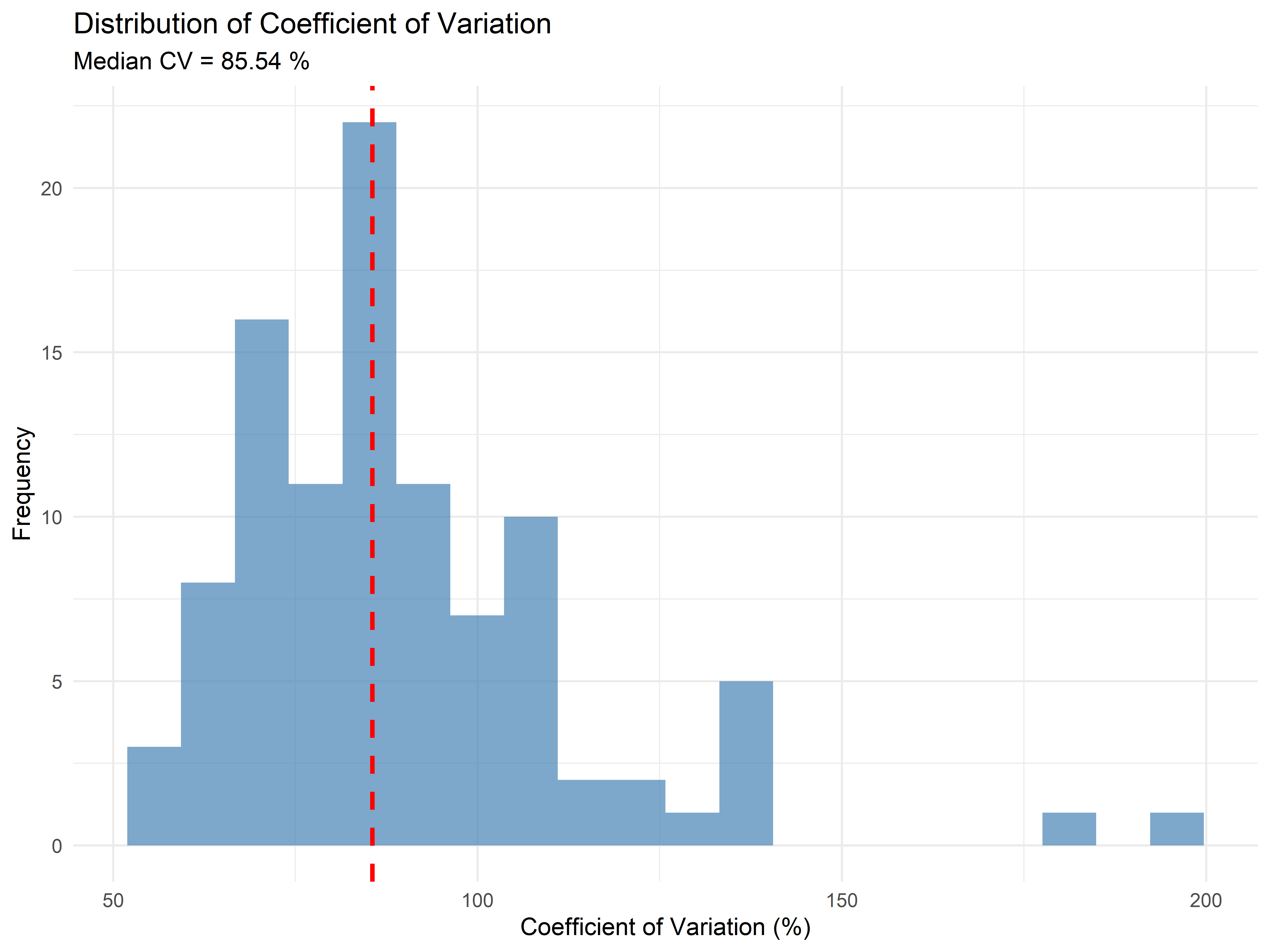
### Distribution Analysis
```{r}
# Analyze distribution of coefficient of variation
ggplot(summary_stats, aes(x = cv)) +
  geom_histogram(bins = 20, fill = "steelblue", alpha = 0.7) +
  geom_vline(xintercept = median(summary_stats$cv),
             color = "red", linetype = "dashed", size = 1) +
  labs(title = "Distribution of Coefficient of Variation",
       subtitle = paste("Median CV =", round(median(summary_stats$cv), 2), "%"),
       x = "Coefficient of Variation (%)", y = "Frequency") +
  theme_minimal()
```
### Analysis-Ready Matrix Check
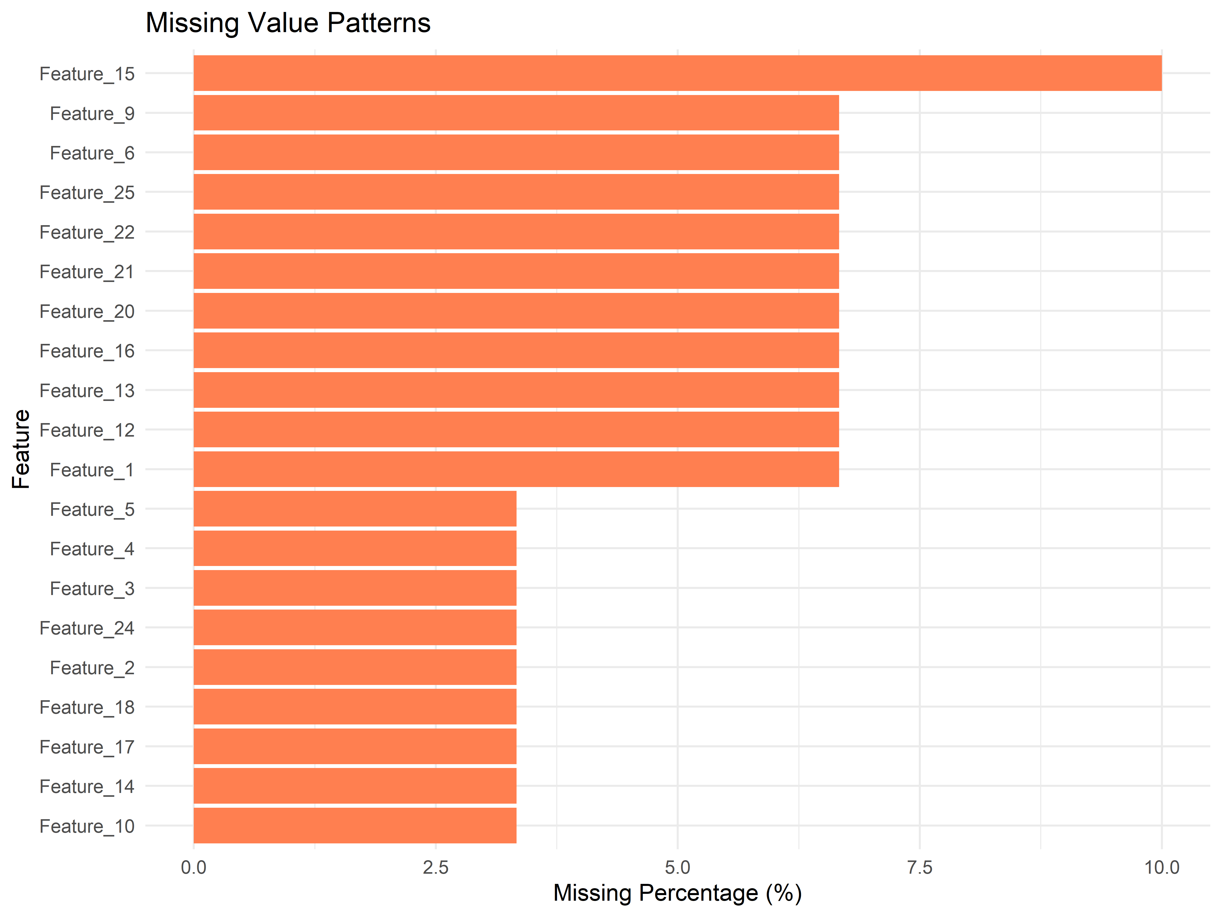
Chapter 18 covers missing-data mechanisms and imputation strategies in detail. At the modeling stage, the goal is only to verify that the matrix passed to the statistical model has the expected feature and sample coverage.
```{r}
# Simulate a small amount of missingness for this modeling example
feature_matrix_with_na <- feature_matrix
missing_indices <- sample(length(feature_matrix), size = length(feature_matrix) * 0.05)
feature_matrix_with_na[missing_indices] <- NA

# Calculate missing value statistics
missing_stats <- data.frame(
  feature = colnames(feature_matrix_with_na),
  missing_count = apply(feature_matrix_with_na, 2, function(x) sum(is.na(x))),
  missing_percent = apply(feature_matrix_with_na, 2, function(x) sum(is.na(x)) / length(x) * 100)
)

# Visualize missing value patterns
missing_pattern <- missing_stats %>%
  filter(missing_count > 0) %>%
  head(20)

if (nrow(missing_pattern) > 0) {
  ggplot(missing_pattern, aes(x = reorder(feature, missing_percent), y = missing_percent)) +
    geom_bar(stat = "identity", fill = "coral") +
    coord_flip() +
    labs(title = "Missing Value Patterns",
         x = "Feature", y = "Missing Percentage (%)") +
    theme_minimal()
}
```
## Hypothesis Testing
### Choosing the Right Test for MS Data
Before running any test, you must answer three questions about your experimental design. The test you choose depends on the answers — and choosing incorrectly either inflates false positives (when assumptions are violated) or wastes statistical power (when a more efficient test exists).
**Question 1: How many groups are you comparing?**
| Groups | Test | R Function | Notes |
|--------|------|-----------|-------|
| **2** | t-test (moderated) | `limma::eBayes()` | Empirical Bayes borrows strength across features |
| **2** (non-normal) | Wilcoxon rank-sum | `wilcox.test()` | Less power; use only when normality is strongly violated |
| **≥ 3** | One-way ANOVA (moderated) | `limma::eBayes()` with multi-level factor | Tests "any difference exists"; follow with contrasts |
| **≥ 3** (non-normal) | Kruskal-Wallis | `kruskal.test()` | Distribution-free; few MS-specific implementations |
**Question 2: Is there a pairing or blocking structure?**
| Design | Approach | Implementation |
|--------|----------|----------------|
| **Unpaired** | Standard two-group comparison | `~ condition` |
| **Paired** (same subject, two conditions) | Block on subject ID | `~ condition + subject` in limma |
| **Blocked** (multiple sites/batches) | Treat blocks as fixed effects | `~ condition + batch` |
| **Repeated measures** | Mixed model with random subject | `lmer(intensity ~ condition + (1|subject))` |
**Question 3: Are there covariates to adjust for?**
| Scenario | Formula Pattern | Rationale |
|----------|----------------|-----------|
| **No covariates** | `~ condition` | Simplest; only valid if randomisation succeeded |
| **Categorical confounder** (e.g., batch) | `~ condition + batch` | Removes batch shift from condition estimate |
| **Continuous covariate** (e.g., age) | `~ condition + age` | Adjusts for linear relationship with age |
| **Interaction** (e.g., treatment × time) | `~ condition * time` | Tests whether treatment effect depends on time |
**The decision tree for MS differential analysis:**
1. **Always start with limma.** Its empirical Bayes moderation was designed for exactly the small-$n$, large-$p$ setting of MS data. A standard t-test with $n = 3$ per group has 2 degrees of freedom — variance estimates are nearly random. limma's shrinkage fixes this.
2. **Add blocking factors for any structure in your design.** If samples were run in batches, add `+ batch` to the design. If the same patient contributed multiple samples, add `+ patient_id`. Omitting blocking factors is the most common cause of false positives in MS differential analysis.
3. **Check the p-value distribution before interpreting results.** A histogram of raw p-values should be uniform above 0.5 (null features) with a peak near 0 (true effects). A U-shaped distribution or a peak near 1 indicates violated assumptions — typically unmodeled correlation or batch effects.
4. **Use FDR, not Bonferroni.** The Bonferroni correction controls the family-wise error rate — appropriate when even one false positive is catastrophic. For MS discovery, FDR at 5 % is the standard.
### Two-Sample t-tests
```{r}
# Perform t-tests for each feature comparing conditions
perform_ttest <- function(feature_data, groups) {
  control_data <- feature_data[groups == "Control"]
  treatment_data <- feature_data[groups == "Treatment"]

  # Check for sufficient data
  if (length(control_data) < 3 || length(treatment_data) < 3) {
    return(data.frame(p.value = NA, statistic = NA, estimate = NA))
  }

  # Perform t-test
  test_result <- t.test(control_data, treatment_data)

  return(data.frame(
    p.value = test_result$p.value,
    statistic = test_result$statistic,
    estimate_diff = test_result$estimate[2] - test_result$estimate[1]
  ))
}

# Apply t-tests to all features
ttest_results <- data.frame()
for (i in 1:ncol(feature_matrix)) {
  result <- perform_ttest(feature_matrix[, i], experimental_data$condition)
  result$feature <- colnames(feature_matrix)[i]
  ttest_results <- rbind(ttest_results, result)
}

# Add multiple testing correction
ttest_results$p.adjusted <- p.adjust(ttest_results$p.value, method = "fdr")

# Display significant results
significant_features <- ttest_results[ttest_results$p.adjusted < 0.05 & !is.na(ttest_results$p.adjusted), ]
cat("Number of significant features (FDR < 0.05):", nrow(significant_features), "\n")
head(significant_features)
```
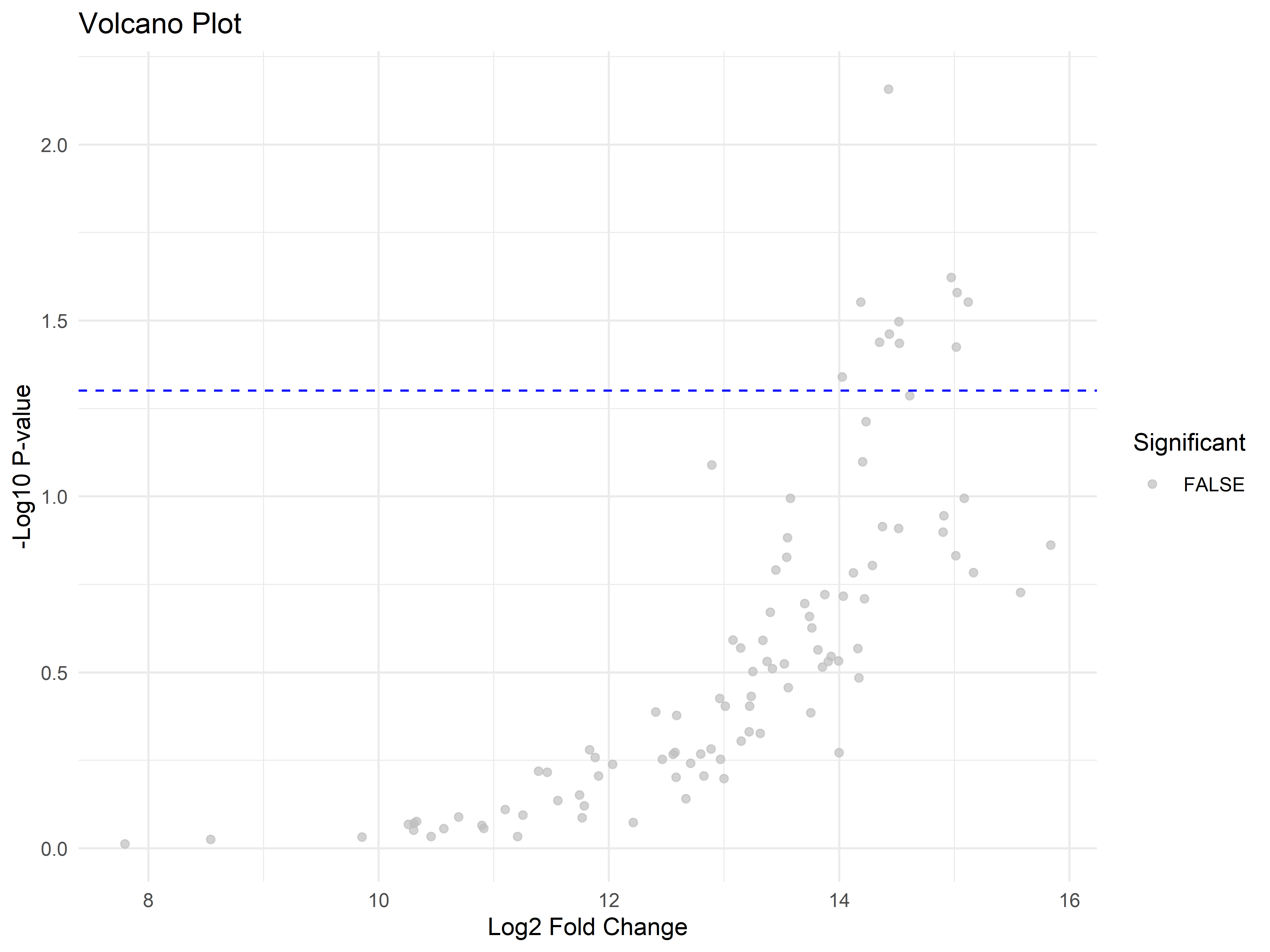
### Volcano Plot
```{r}
# Create volcano plot
volcano_data <- ttest_results %>%
  mutate(
    log2_fold_change = log2(abs(estimate_diff) + 1),  # Add 1 to avoid log(0)
    neg_log10_p = -log10(p.value),
    significant = p.adjusted < 0.05 & !is.na(p.adjusted)
  )

ggplot(volcano_data, aes(x = log2_fold_change, y = neg_log10_p)) +
  geom_point(aes(color = significant), alpha = 0.7) +
  scale_color_manual(values = c("FALSE" = "gray", "TRUE" = "red")) +
  geom_hline(yintercept = -log10(0.05), linetype = "dashed", color = "blue") +
  labs(title = "Volcano Plot",
       x = "Log2 Fold Change", y = "-Log10 P-value",
       color = "Significant") +
  theme_minimal()
```
## ANOVA for Multiple Groups
```{r}
# Add a third condition for ANOVA demonstration
experimental_data_extended <- rbind(
  experimental_data,
  data.frame(
    condition = rep("Treatment2", 10),
    timepoint = rep("T0", 10),
    replicate = rep(1:5, 2),
    sample_id = paste0("S", (nrow(experimental_data) + 1):(nrow(experimental_data) + 10)),
    batch = rep(1:2, each = 5)
  )
)

# Extend feature matrix
additional_samples <- matrix(
  rlnorm(10 * n_features, meanlog = 10.2, sdlog = 1),
  nrow = 10,
  ncol = n_features
)
colnames(additional_samples) <- colnames(feature_matrix)
rownames(additional_samples) <- experimental_data_extended$sample_id[31:40]

feature_matrix_extended <- rbind(feature_matrix, additional_samples)

# Perform one-way ANOVA for each feature
perform_anova <- function(feature_data, groups) {
  if (length(unique(groups)) < 2) return(data.frame(p.value = NA, f.statistic = NA))

  anova_result <- aov(feature_data ~ groups)
  summary_result <- summary(anova_result)

  return(data.frame(
    p.value = summary_result[[1]][1, "Pr(>F)"],
    f.statistic = summary_result[[1]][1, "F value"]
  ))
}

# Apply ANOVA to all features
anova_results <- lapply(1:ncol(feature_matrix_extended), function(i) {
  result <- perform_anova(feature_matrix_extended[, i], experimental_data_extended$condition)
  result$feature <- colnames(feature_matrix_extended)[i]
  return(result)
})
anova_results <- do.call(rbind, anova_results)

# Add multiple testing correction
anova_results$p.adjusted <- p.adjust(anova_results$p.value, method = "fdr")

# Display significant ANOVA results
significant_anova <- anova_results[anova_results$p.adjusted < 0.05 & !is.na(anova_results$p.adjusted), ]
cat("Number of significant features (ANOVA FDR < 0.05):", nrow(significant_anova), "\n")
```
## Correlation Analysis
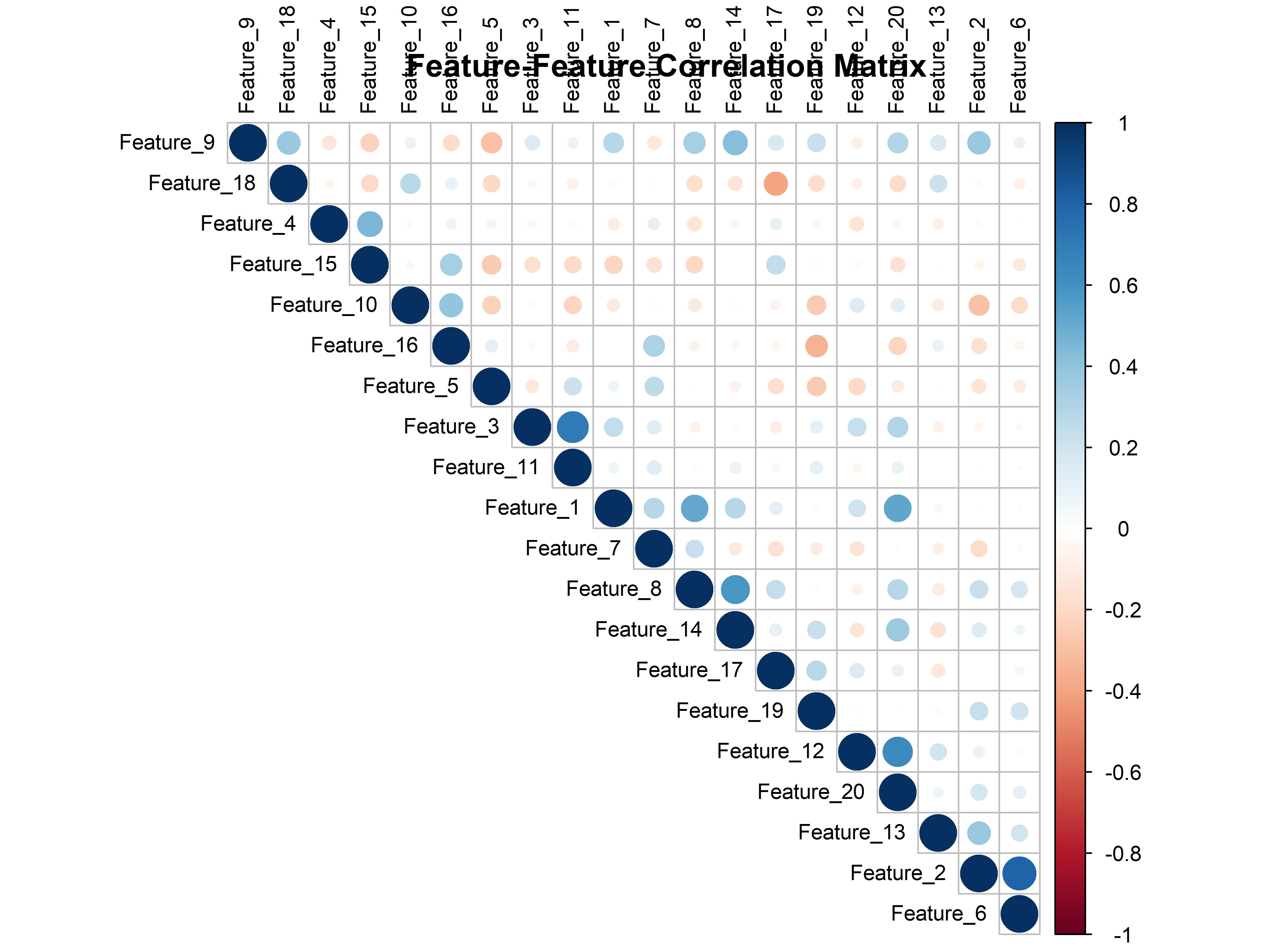
### Feature-Feature Correlations
```{r}
# Calculate correlation matrix for a subset of features
feature_subset <- feature_matrix[, 1:20]  # Use subset for visualization
cor_matrix <- cor(feature_subset, use = "complete.obs")

# Visualize correlation matrix
corrplot(cor_matrix, method = "circle", type = "upper",
         order = "hclust", tl.cex = 0.8, tl.col = "black")
title("Feature-Feature Correlation Matrix")
```
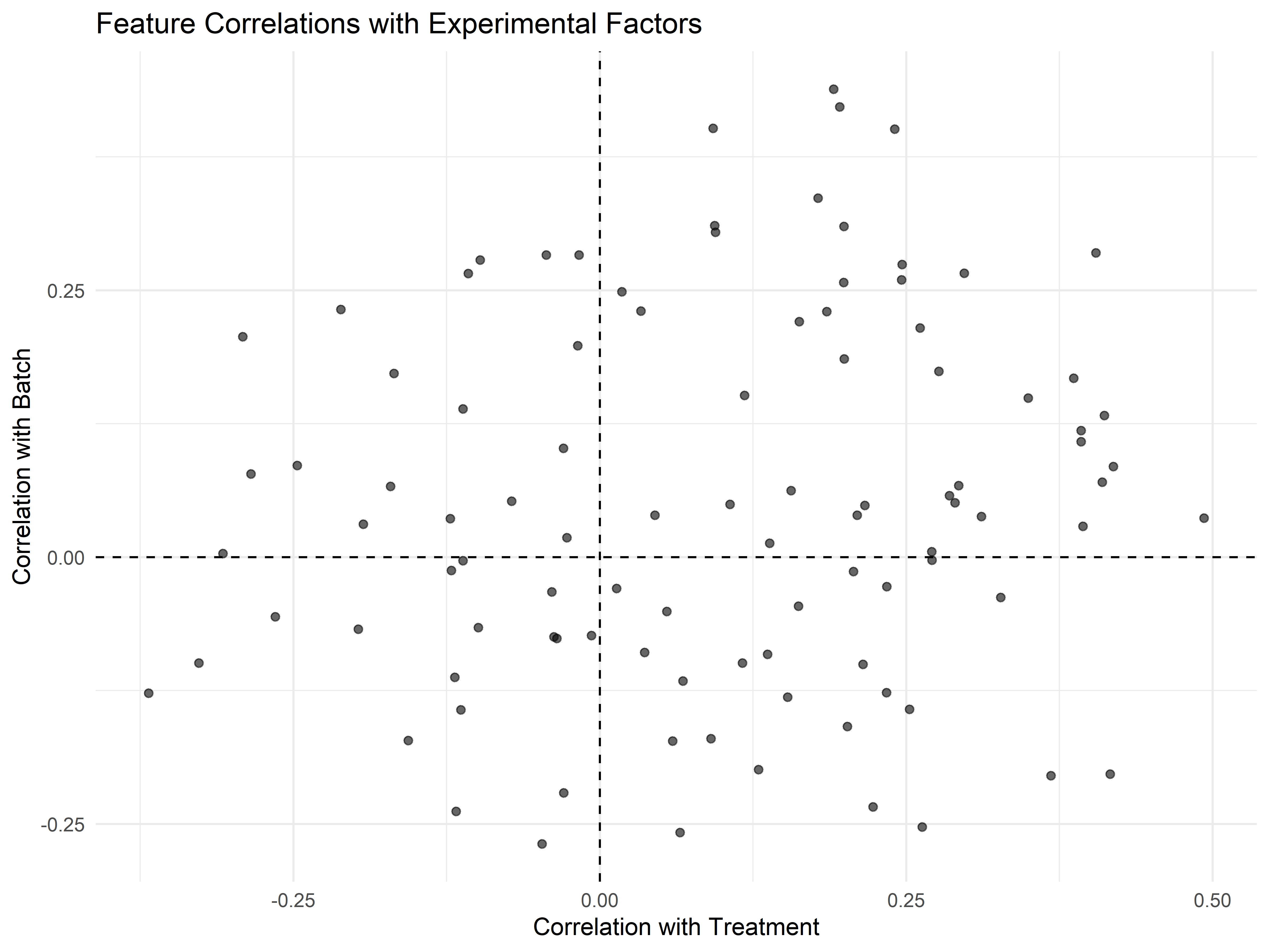
### Correlation with Experimental Factors
```{r}
# Encode experimental factors as numeric for correlation
experimental_numeric <- experimental_data %>%
  mutate(
    condition_numeric = ifelse(condition == "Control", 0, 1),
    batch_numeric = as.numeric(batch)
  )

# Calculate correlations between features and experimental factors
cor_with_condition <- apply(feature_matrix, 2, function(x) {
  cor(x, experimental_numeric$condition_numeric, use = "complete.obs")
})

cor_with_batch <- apply(feature_matrix, 2, function(x) {
  cor(x, experimental_numeric$batch_numeric, use = "complete.obs")
})

# Visualize correlations
correlation_df <- data.frame(
  feature = names(cor_with_condition),
  condition_cor = cor_with_condition,
  batch_cor = cor_with_batch
)

ggplot(correlation_df, aes(x = condition_cor, y = batch_cor)) +
  geom_point(alpha = 0.6) +
  geom_hline(yintercept = 0, linetype = "dashed") +
  geom_vline(xintercept = 0, linetype = "dashed") +
  labs(title = "Feature Correlations with Experimental Factors",
       x = "Correlation with Treatment", y = "Correlation with Batch") +
  theme_minimal()
```
## Principal Component Analysis (PCA)
### Performing PCA
```{r}
# Standardize data for PCA
feature_matrix_scaled <- scale(feature_matrix)

# Perform PCA
pca_result <- prcomp(feature_matrix_scaled, center = FALSE, scale. = FALSE)

# Extract PC scores
pca_scores <- data.frame(pca_result$x) %>%
  mutate(
    sample_id = experimental_data$sample_id,
    condition = experimental_data$condition,
    batch = factor(experimental_data$batch)
  )

# Variance explained
variance_explained <- (pca_result$sdev^2) / sum(pca_result$sdev^2) * 100
```
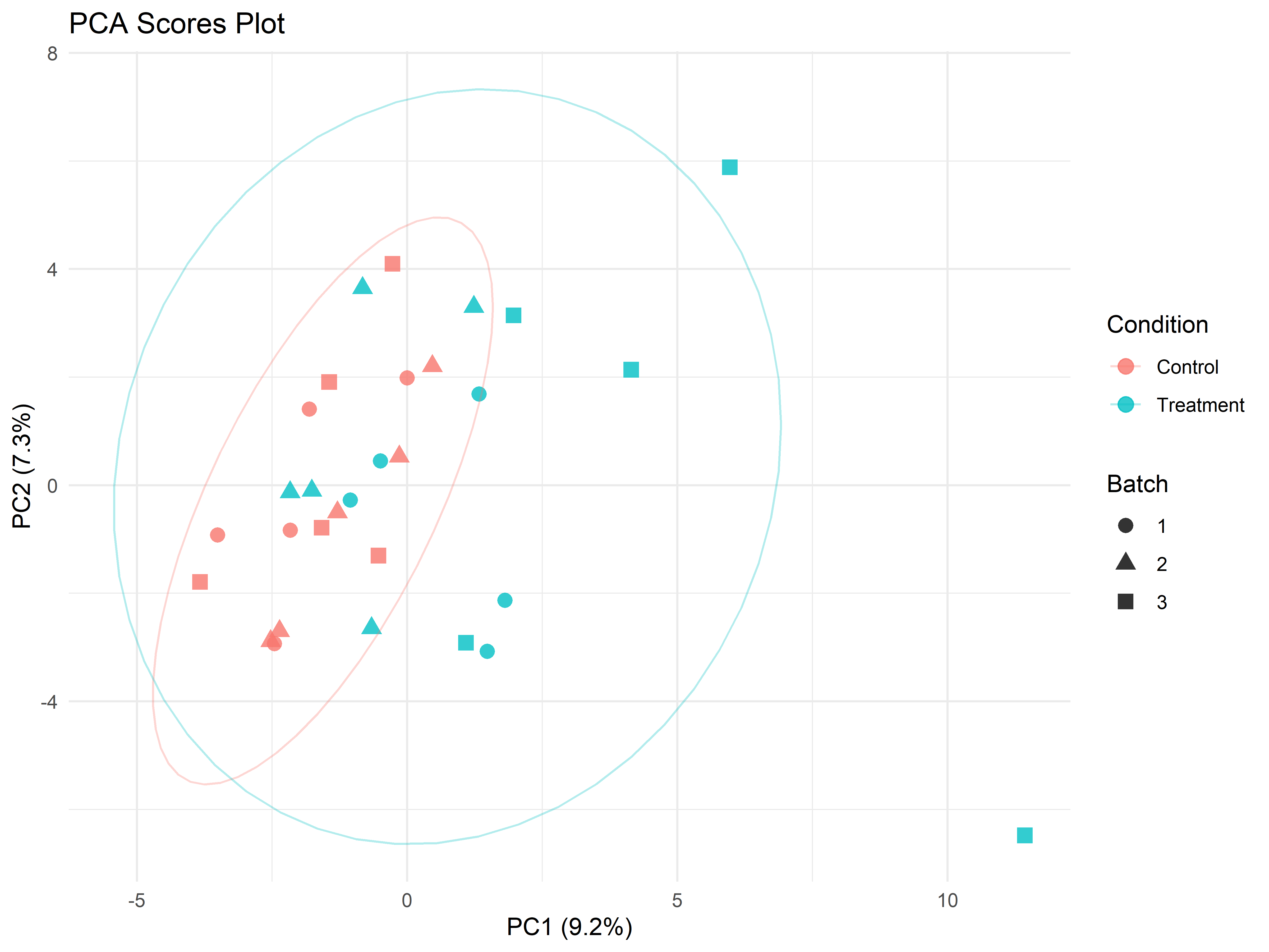
### PCA Visualization
```{r}
# PCA scores plot
ggplot(pca_scores, aes(x = PC1, y = PC2, color = condition, shape = batch)) +
  geom_point(size = 3, alpha = 0.8) +
  stat_ellipse(aes(group = condition), alpha = 0.3) +
  labs(title = "PCA Scores Plot",
       x = paste0("PC1 (", round(variance_explained[1], 1), "%)"),
       y = paste0("PC2 (", round(variance_explained[2], 1), "%)"),
       color = "Condition", shape = "Batch") +
  theme_minimal()
```
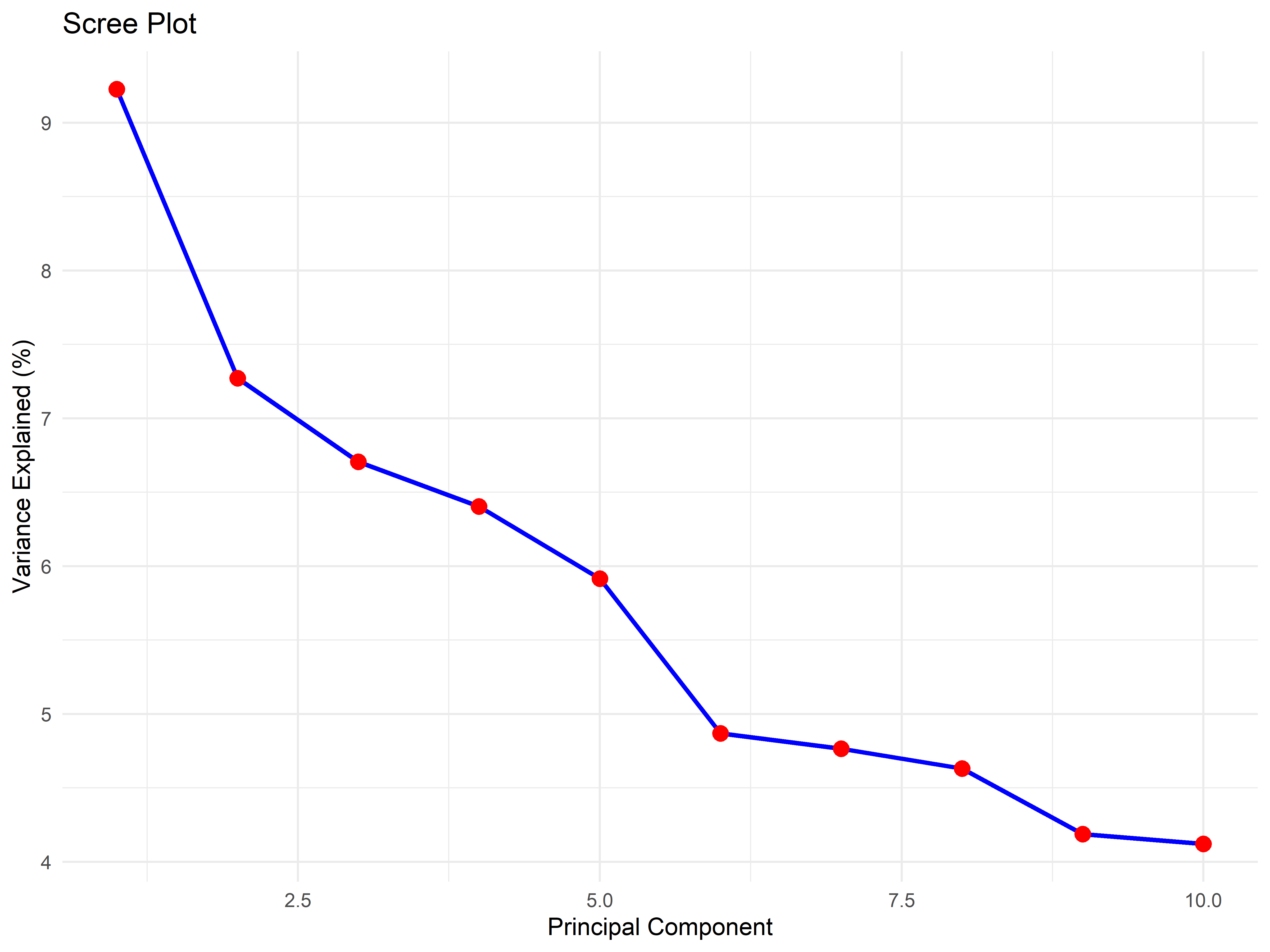
### Scree Plot
```{r}
# Scree plot
scree_data <- data.frame(
  PC = 1:min(10, length(variance_explained)),
  Variance = variance_explained[1:min(10, length(variance_explained))]
)

ggplot(scree_data, aes(x = PC, y = Variance)) +
  geom_line(color = "blue", size = 1) +
  geom_point(color = "red", size = 3) +
  labs(title = "Scree Plot",
       x = "Principal Component", y = "Variance Explained (%)") +
  theme_minimal()
```
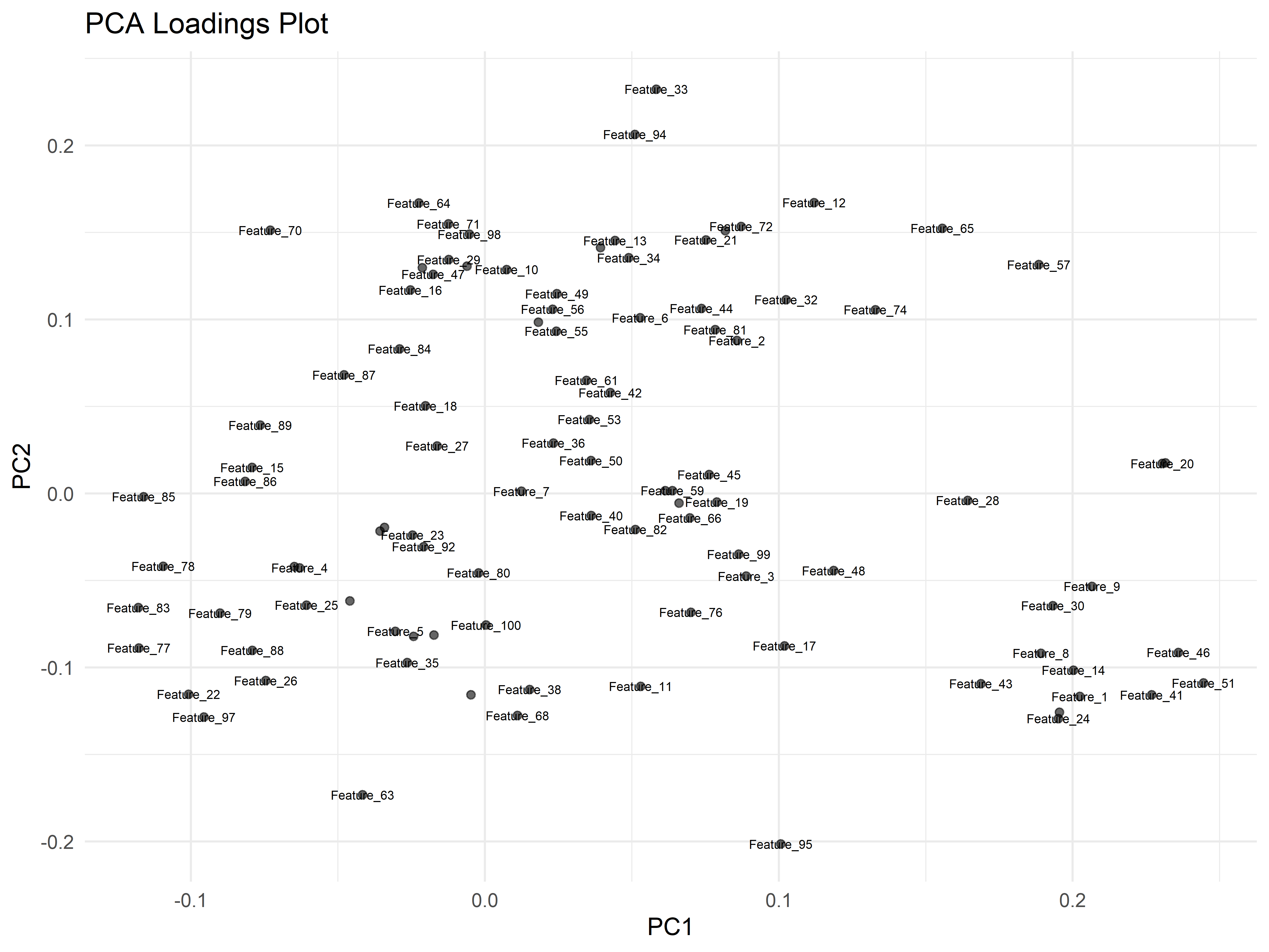
### PCA Loadings
```{r}
# Extract and visualize loadings
loadings_data <- data.frame(
  feature = colnames(feature_matrix),
  PC1 = pca_result$rotation[, 1],
  PC2 = pca_result$rotation[, 2]
)

# Plot loadings
ggplot(loadings_data, aes(x = PC1, y = PC2)) +
  geom_point(alpha = 0.6) +
  geom_text(aes(label = feature), size = 2, check_overlap = TRUE) +
  labs(title = "PCA Loadings Plot",
       x = "PC1", y = "PC2") +
  theme_minimal()
```
## Clustering Analysis
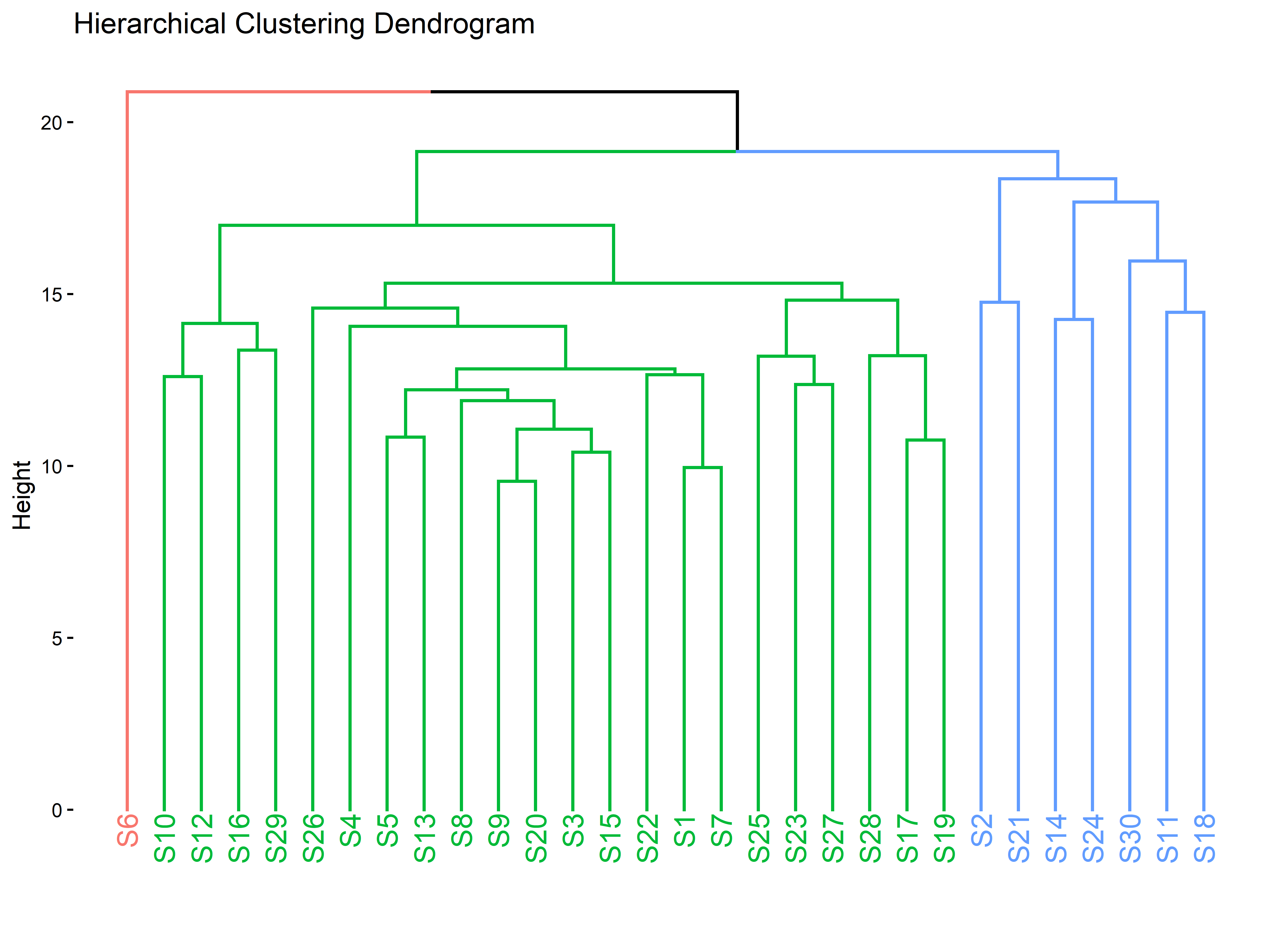
### Hierarchical Clustering
```{r}
# Perform hierarchical clustering
dist_matrix <- dist(feature_matrix_scaled)
hclust_result <- hclust(dist_matrix, method = "ward.D2")

# Cut tree to get clusters
n_clusters <- 3
cluster_assignments <- cutree(hclust_result, k = n_clusters)

# Add cluster assignments to experimental data
experimental_data$cluster <- factor(cluster_assignments)

# Visualize dendrogram
if (factoextra_available) {
  factoextra::fviz_dend(
    hclust_result,
    k = n_clusters,
    cex = 0.8,
    color_labels_by_k = TRUE,
    main = "Hierarchical Clustering Dendrogram"
  )
} else {
  plot(hclust_result, labels = FALSE, main = "Hierarchical Clustering Dendrogram")
  rect.hclust(hclust_result, k = n_clusters, border = 2:4)
}
```
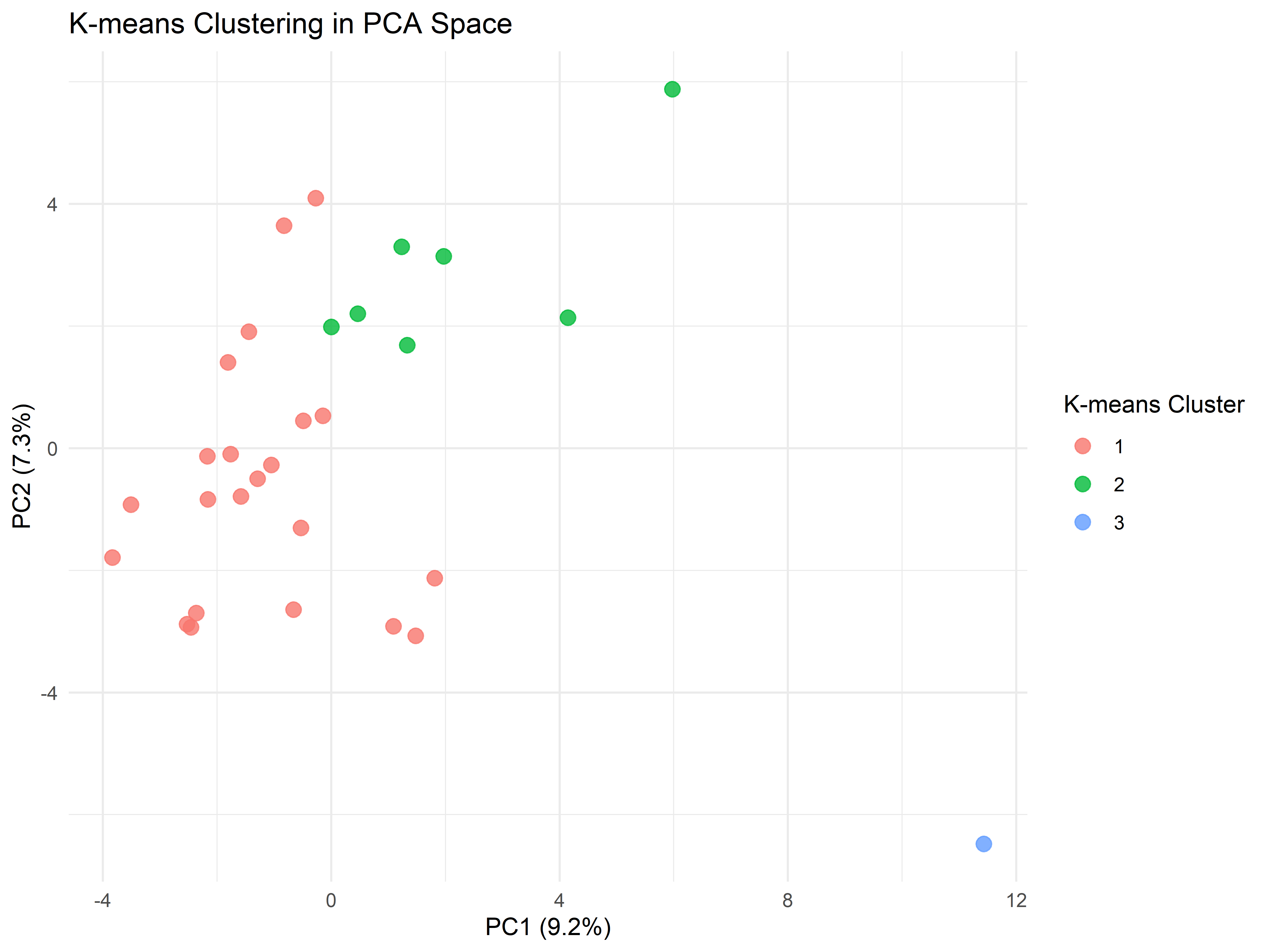
### K-means Clustering
```{r}
# Perform k-means clustering
set.seed(123)
kmeans_result <- kmeans(feature_matrix_scaled, centers = 3, nstart = 25)

# Add k-means clusters to data
experimental_data$kmeans_cluster <- factor(kmeans_result$cluster)

# Visualize clusters in PCA space
ggplot(pca_scores, aes(x = PC1, y = PC2)) +
  geom_point(aes(color = experimental_data$kmeans_cluster), size = 3, alpha = 0.8) +
  labs(title = "K-means Clustering in PCA Space",
       x = paste0("PC1 (", round(variance_explained[1], 1), "%)"),
       y = paste0("PC2 (", round(variance_explained[2], 1), "%)"),
       color = "K-means Cluster") +
  theme_minimal()
```
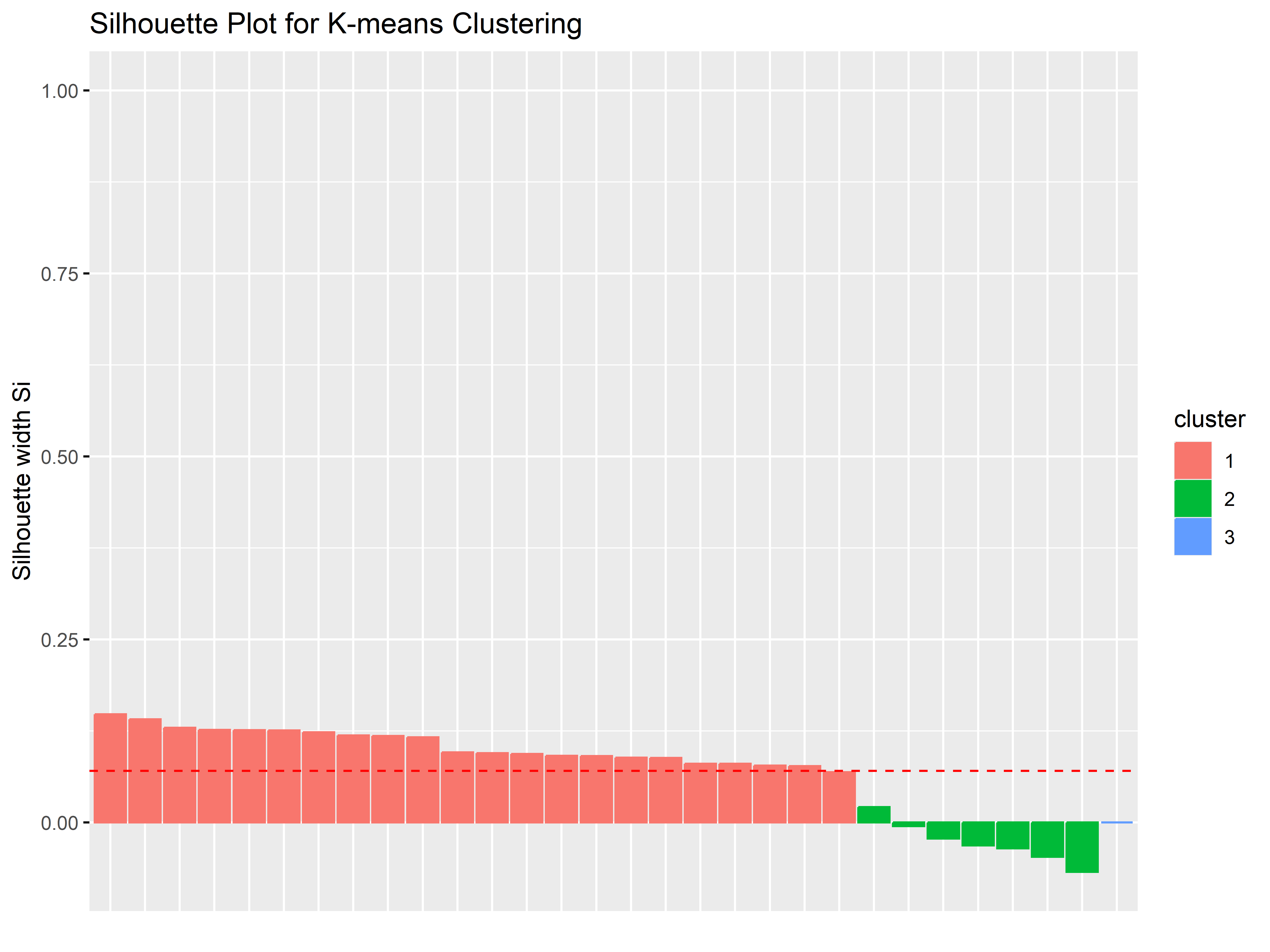
### Cluster Validation
```{r}
# Silhouette analysis
sil_scores <- silhouette(kmeans_result$cluster, dist_matrix)

# Visualize silhouette plot
if (factoextra_available) {
  factoextra::fviz_silhouette(
    sil_scores,
    main = "Silhouette Plot for K-means Clustering"
  )
} else {
  plot(sil_scores, main = "Silhouette Plot for K-means Clustering")
}
# Average silhouette width
avg_sil_width <- mean(sil_scores[, 3])
cat("Average silhouette width:", round(avg_sil_width, 3), "\n")
```
## Heat Map Analysis
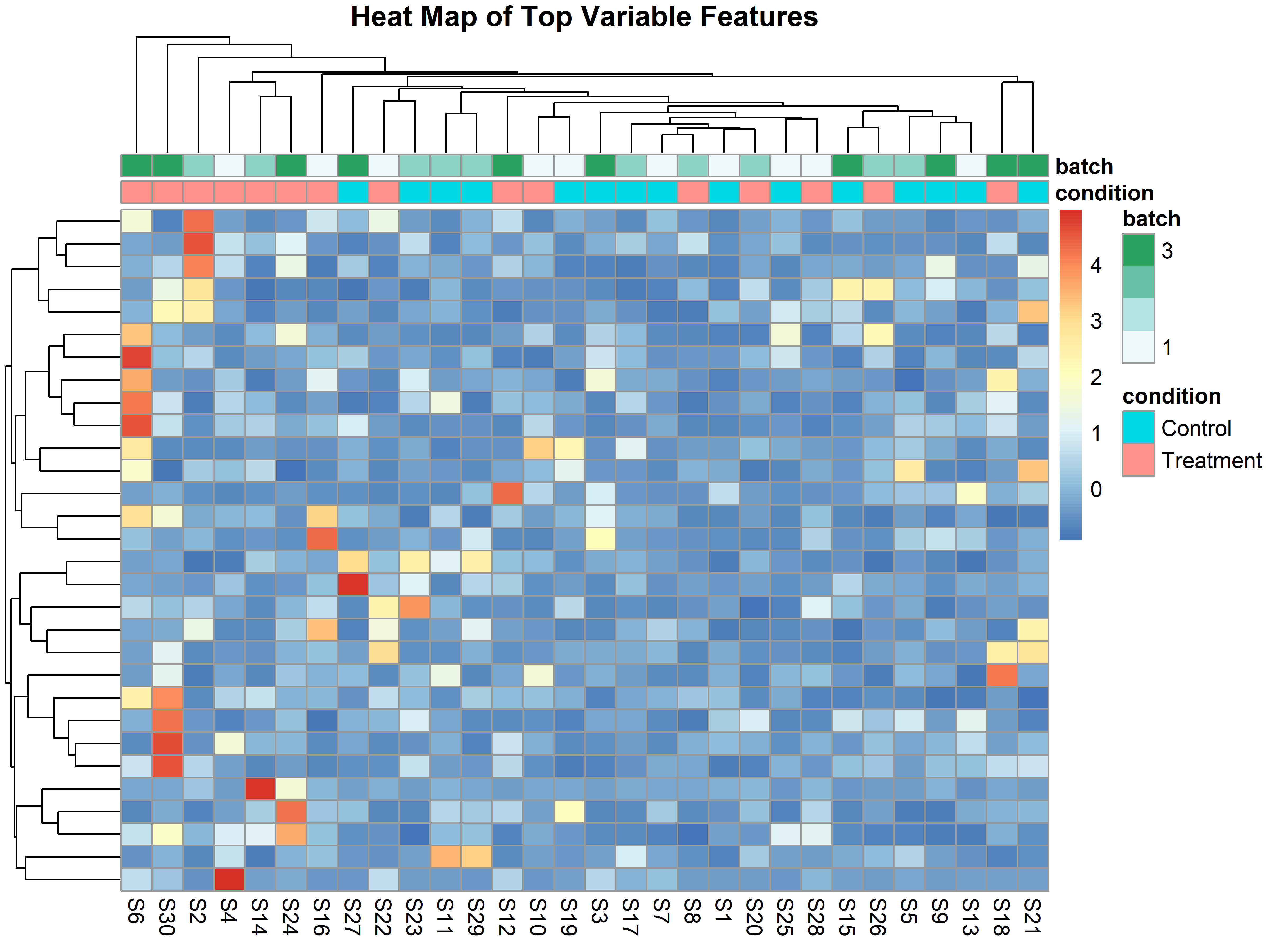
### Feature Heat Map
```{r}
# Create heat map of top variable features
top_variable_features <- summary_stats %>%
  top_n(30, cv) %>%
  pull(feature)

heatmap_data <- feature_matrix[, top_variable_features]

# Create annotation for samples
annotation_df <- experimental_data %>%
  select(condition, batch) %>%
  data.frame(row.names = experimental_data$sample_id)

# Generate heat map
pheatmap(t(scale(heatmap_data)),
         annotation_col = annotation_df,
         show_rownames = FALSE,
         show_colnames = TRUE,
         clustering_distance_rows = "euclidean",
         clustering_distance_cols = "euclidean",
         main = "Heat Map of Top Variable Features")
```
## Choosing a Differential Abundance Method
This chapter develops `limma` as the primary framework because it builds directly on the design-matrix, contrast, and empirical-Bayes reasoning that the chapter already covers. `limma` is battle-tested, flexible, and well-suited to the small-sample, many-feature setting of mass spectrometry [@ritchie2015limma]. However, the proteomics and metabolomics landscape offers several alternative tools, each making distinct trade-offs about input level, missing-data handling, variance modelling, and supported designs. This section helps you navigate those trade-offs so you can choose the right tool for a given experiment — and understand why different tools sometimes give different answers.
### Decision Table of Differential Abundance Methods
The table below compares eight widely used packages across the dimensions that matter most for MS data: input requirements, missing-value strategy, variance modelling, design complexity, and typical use cases.
| Package/Workflow | Expected Input Level | Aggregation Included? | Missing-Value Strategy | Variance/Model Strategy | Supported Design Complexity | Strongest Use Case | Principal Limitation |
|---|---|---|---|---|---|---|---|
| `limma` | Protein (or feature) matrix | No | Requires complete matrix; imputation upstream | Empirical Bayes moderation across all features | Two-group, factorial, blocking, continuous covariates | General-purpose differential testing with flexible design matrices | No native handling of missing values or peptide-level uncertainty |
| `DEP` | Protein (MaxQuant / `QFeatures`) | No (peptide-to-protein upstream) | Left-censored imputation (`MinProb`, `QRILC`, `knn`) | Wraps `limma` empirical Bayes; includes VSN normalization | Two-group, multi-group via contrasts | End-to-end LFQ differential pipeline from protein table to volcano plot | Limited to protein-group tables; design flexibility constrained by wrapper |
| `MSstats` | Peptide (not protein) | Yes (run-level summarization) | Missing features excluded per protein; handles unbalanced data | Linear mixed model per protein; model-based shrinkage | Time-course, group comparison, labelled/unlabelled | Peptide-to-protein inference with uncertainty propagation | Model per protein can be slow with thousands of features |
| `msqrob2` | Peptide or protein | Yes (robust summarization workflows) | Hurdle model for missingness without imputation; or robust ridge regression | Robust ridge regression + empirical Bayes; or hurdle mixed-model workflow | Two-group, multi-group, factorial | Flexible workflows: robust for outliers, hurdle for missing-heavy data | Two workflow paths (robust vs. hurdle) require user awareness of trade-offs |
| `proDA` | Protein (LFQ intensities) | No | Probabilistic dropout model; no imputation needed | Empirical Bayes with location and scale moderation | Two-group, multi-group, linear models | Label-free proteomics with substantial missing values | Designed for LFQ only; not applicable to TMT or targeted data |
| `DEqMS` | Protein (with peptide/PSM counts) | No (peptide count from upstream) | Requires complete matrix; imputation upstream | Prior variance scaled by peptide/PSM count per protein (`spectraCounteBayes`) | Two-group, multi-group, factorial | Correcting variance estimation for proteins quantified by few peptides | Requires peptide/PSM count column; does not aggregate PSMs to proteins |
| `limpa` | Peptide/precursor (not protein) | Yes (DPC-Quant probabilistic quantification) | Detection-probability curve (DPC) models missingness; no imputation | Empirical Bayes precision weights via `vooma`; full limma downstream | Any design matrix supported by `limma` | Precursor-level quantification with information recovery from missing values | Relatively new (2025); community adoption still growing |
| `PolySTest` | Protein (or feature) matrix | No | Combines quantitative evidence with missingness patterns in one test | Combined p-value from quantitative test + missingness test | Two-group (limited replicates) | Low-replication settings (< 4 replicates) where missingness carries signal | Limited to two-group comparisons; complex designs need other tools |
::: {.callout-note title="Correcting Common Misconceptions"}
The methods above are sometimes misunderstood in practice. Here are the key distinctions:
- **`DEqMS` adjusts the prior variance using peptide/PSM counts** — it does NOT aggregate PSMs to proteins. You must supply a protein-summarized matrix plus the number of PSMs or peptides that quantified each protein. Without a PSM/peptide-count column, `DEqMS` cannot function.
- **`proDA` targets label-free proteomics specifically** and models probabilistic dropout without any imputation step. The sigmoidal dropout curve captures intensity-dependent missingness, and empirical Bayes priors shrink both location and scale estimates.
- **`msqrob2` provides robust ridge regression AND hurdle/mixed-model workflows** — the former down-weights outlier peptides, the latter models missingness directly without imputation. Which path to use depends on whether your data has many outliers or many missing values.
- **`PolySTest` combines quantitative and missingness evidence** into a single test statistic, making it especially powerful in low-replication settings where a feature missing in all replicates of one condition but detected in all replicates of the other is strong evidence.
- **`limpa` combines detection-probability-based quantification (DPC-Quant) with limma-style differential analysis.** It recovers information from missing precursor intensities without imputation by modelling the probability that each precursor is detected, then propagates the uncertainty into precision weights.
:::
### Decision Tree
The following mermaid diagram guides you from your experimental design and input level to an appropriate method. Start at the top and follow the branch that matches your data.
```{mermaid}
%%| fig-width: 10
%%| fig-height: 8
flowchart TD
    Start["What is your input level?"]
    Start --> Peptide["Peptide/precursor intensities"]
    Start --> Protein["Protein-level matrix"]

    Peptide --> MSstats["MSstats<br/>(linear mixed model,<br/>run-level summarization)"]
    Peptide --> msqrob2P["msqrob2<br/>(robust ridge or<br/>hurdle workflow)"]
    Peptide --> limpa["limpa<br/>(DPC-Quant +<br/>probabilistic dropout)"]

    Protein --> Miss["Do you have<br/>substantial missing values?"]
    Miss -->|"Yes"| RepLow["Few replicates<br/>(< 4 per group)?"]
    Miss -->|"No / minimal"| Variance["Do peptide/PSM counts<br/>vary widely?"]

    RepLow -->|"Yes"| PolySTest["PolySTest<br/>(combined quant +<br/>missingness test)"]
    RepLow -->|"No (≥ 4)"| proDA["proDA<br/>(probabilistic dropout,<br/>no imputation)"]

    Variance -->|"Yes"| DEqMS["DEqMS<br/>(variance adjusted by<br/>peptide/PSM count)"]
    Variance -->|"No"| LimmaStraight["limma<br/>(flexible design,<br/>empirical Bayes)"]

    LimmaStraight --> DEP["DEP<br/>(wraps limma +<br/>built-in pipeline)"]
    msqrob2P --> msqrob2W["msqrob2<br/>(hurdle workflow<br/>if missing; robust<br/>if outliers)"]
```
### Comparison Example: limma vs. proDA
The choice of method matters in practice. To illustrate, we compare `limma` (with standard preprocessing) against `proDA` (which handles missing values probabilistically) on the `DEP::UbiLength` dataset [@zhang2018dep], testing the Ubi1 condition against the Ctrl condition.
```{r}
#| eval: false
library(DEP)
library(limma)
library(proDA)
library(tidyverse)

# ---- Load and prepare data ----
data("UbiLength", package = "DEP")
data("UbiLength_ExpDesign", package = "DEP")

protein_clean <- UbiLength |>
  filter(Reverse != "+", Potential.contaminant != "+")

# Select LFQ columns
lfq_cols <- grep("^LFQ\\.intensity\\.", colnames(protein_clean))

# ---- limma pipeline (preprocessing + empirical Bayes) ----
se <- make_se(protein_clean, lfq_cols, UbiLength_ExpDesign)
se_filt <- filter_missval(se, thr = 0)
se_norm <- normalize_vsn(se_filt)
set.seed(1)
se_imp <- impute(se_norm, fun = "MinProb", q = 0.01)

se_diff <- test_diff(se_imp, type = "control", control = "Ctrl")
limma_results <- get_results(se_diff) |>
  rownames_to_column("protein") |>
  select(protein, contains("Ubi1_vs_Ctrl"))

# ---- proDA pipeline (probabilistic dropout, no imputation) ----
# Build raw log2 matrix
lfq_matrix <- protein_clean[, lfq_cols]
colnames(lfq_matrix) <- UbiLength_ExpDesign$label
raw_log2 <- log2(as.matrix(lfq_matrix))
raw_log2[is.infinite(raw_log2)] <- NA

# Filter features with excessive missingness
keep <- rowSums(is.na(raw_log2)) < ncol(raw_log2) * 0.8
raw_log2 <- raw_log2[keep, ]
protein_names <- protein_clean$Gene.names[keep]

col_data <- UbiLength_ExpDesign |>
  mutate(condition = factor(condition)) |>
  column_to_rownames("label")

# Fit proDA model and test
proda_fit <- proDA(raw_log2, design = ~ condition)
proda_results <- test_diff(proda_fit,
  contrast = "conditionUbi1 - conditionCtrl") |>
  as.data.frame() |>
  rownames_to_column("protein") |>
  mutate(protein = protein_names[match(protein, rownames(raw_log2))])

# ---- Compare results ----
comparison <- inner_join(
  limma_results |>
    select(protein, lfc_limma = Ubi1_vs_Ctrl_ratio,
           p_limma = Ubi1_vs_Ctrl_p.adj),
  proda_results |>
    select(protein, lfc_proda = log2FoldChange,
           p_proda = adj_pval),
  by = "protein"
)

# Effect-size concordance
cor_log2FC <- cor(comparison$lfc_limma, comparison$lfc_proda,
                  use = "complete.obs")
cat("Pearson correlation of log2 fold changes:",
    round(cor_log2FC, 3), "\n")

# Discovery overlap at 5% FDR
n_limma <- sum(comparison$p_limma < 0.05, na.rm = TRUE)
n_proda <- sum(comparison$p_proda < 0.05, na.rm = TRUE)
n_both <- sum(comparison$p_limma < 0.05 & comparison$p_proda < 0.05,
              na.rm = TRUE)

cat("Discoveries at 5% FDR:\n")
cat("  limma:", n_limma, "\n")
cat("  proDA:", n_proda, "\n")
cat("  Overlap:", n_both, "\n")
```
The results typically show high concordance in log2 fold change estimates (Pearson correlation > 0.9), but the number of discoveries can differ. `proDA` often detects additional features that `limma` discards during missing-value filtering, especially those with moderate fold changes in proteins quantified by few peptides. Conversely, `limma` may call features significant that `proDA` down-weights because their dropout pattern suggests low confidence. This divergence is informative: features significant in only one method warrant closer inspection of their raw intensity profiles.
::: {.callout-warning title="Do Not Shop for Significant Results"}
Method choice must be specified before looking at which method yields more significant results. Choosing a method post hoc — based on which one returns a more "desirable" list of hits — inflates false positives and renders downstream biological interpretation unreliable. Pre-register your analysis pipeline, or at minimum document your decision process before running the differential test.
:::
## Example 1: Label-Free Proteomics Differential Protein Abundance
### Project Question
Which proteins are differentially abundant between biological conditions in a label-free proteomics experiment?
This is the first full real-data example because it joins the main decisions introduced across the previous chapters: identification-derived protein tables, missingness, normalization, differential abundance, visualization, interpretation, and reproducible export.
### Dataset and Scope
This example uses `DEP::UbiLength`, a MaxQuant-style LFQ protein-group table, together with `DEP::UbiLength_ExpDesign`, the matching experimental design. The design contains 12 samples across 4 conditions with 3 replicates per condition.
Raw mzML-level QC is not the focus here because `UbiLength` starts from a processed protein table. Instead, the defensible QC layer is matrix-level QC: sample intensity distributions, missingness, PCA, sample distances, and inspection of significant proteins after modeling.
### Workflow Map
| Step | Implementation |
|---|---|
| Metadata and contrasts | Use `UbiLength_ExpDesign`; compare each ubiquitin condition against `Ctrl` |
| Processed table import | Load `DEP::UbiLength`, a MaxQuant-style proteinGroups table |
| Identification audit | Remove reverse hits and potential contaminants |
| Abundance object | Build a `SummarizedExperiment` with LFQ intensity columns |
| Missingness filtering | Use `DEP::filter_missval()` before normalization |
| Normalization | Use `DEP::normalize_vsn()` |
| Imputation | Use left-censored imputation only after missingness diagnostics |
| Statistical modeling | Use `DEP::test_diff()`, backed by limma-style empirical Bayes modeling |
| Multiple testing | Use adjusted p-values/FDR in DEP result tables |
| Visualization | PCA, volcano plot, MA plot, heatmap |
| Interpretation | Prepare significant proteins for GO or Reactome enrichment |
| Reproducible export | Save tables, figures, R objects, and session information |
### Setup
The code below is marked `eval: false` because it is intended as a complete book-style analysis script. It may install or require optional packages that are not needed for rendering this chapter.
```{r}
#| eval: false
if (!requireNamespace("BiocManager", quietly = TRUE)) {
  install.packages("BiocManager")
}

bioc_pkgs <- c(
  "DEP",
  "SummarizedExperiment",
  "limma",
  "vsn",
  "ComplexHeatmap",
  "clusterProfiler",
  "ReactomePA",
  "org.Sc.sgd.db"
)

cran_pkgs <- c(
  "tidyverse",
  "janitor",
  "naniar",
  "ggrepel",
  "patchwork",
  "here",
  "sessioninfo"
)

for (pkg in bioc_pkgs) {
  if (!requireNamespace(pkg, quietly = TRUE)) {
    BiocManager::install(pkg, ask = FALSE, update = FALSE)
  }
}

for (pkg in cran_pkgs) {
  if (!requireNamespace(pkg, quietly = TRUE)) {
    install.packages(pkg, repos = "https://cloud.r-project.org")
  }
}

library(DEP)
library(SummarizedExperiment)
library(limma)
library(vsn)
library(tidyverse)
library(janitor)
library(naniar)
library(ggrepel)
library(patchwork)
library(sessioninfo)
```
### Load Data and Metadata
```{r}
#| eval: false
dir.create("results", showWarnings = FALSE)
dir.create("figures", showWarnings = FALSE)
dir.create("objects", showWarnings = FALSE)

data("UbiLength", package = "DEP")
data("UbiLength_ExpDesign", package = "DEP")

protein_raw <- UbiLength
exp_design <- UbiLength_ExpDesign |>
  as_tibble() |>
  mutate(
    label = as.character(label),
    condition = factor(condition),
    replicate = factor(replicate)
  )

dim(protein_raw)
exp_design
table(exp_design$condition)
```
### Audit Identifications and Build the Abundance Object
```{r}
#| eval: false
protein_clean <- protein_raw |>
  filter(Reverse != "+", Potential.contaminant != "+")

protein_unique <- make_unique(
  protein_clean,
  names = "Gene.names",
  ids = "Protein.IDs",
  delim = ";"
)

lfq_cols <- grep("^LFQ\\.intensity\\.", colnames(protein_unique))

se <- make_se(
  proteins_unique = protein_unique,
  columns = lfq_cols,
  expdesign = exp_design
)

saveRDS(se, "objects/01_ubilength_se_raw.rds")
se
```
### Matrix-Level QC and Missingness
```{r}
#| eval: false
p_numbers <- plot_numbers(se)
p_coverage <- plot_coverage(se)
p_missval <- plot_missval(se)

ggsave("figures/dep_01_protein_numbers.png", p_numbers, width = 7, height = 5, dpi = 300)
ggsave("figures/dep_02_protein_coverage.png", p_coverage, width = 7, height = 5, dpi = 300)
ggsave("figures/dep_03_missing_values.png", p_missval, width = 7, height = 6, dpi = 300)

assay_raw <- assay(se)
missing_summary <- tibble(
  sample = colnames(assay_raw),
  n_missing = colSums(is.na(assay_raw)),
  pct_missing = colMeans(is.na(assay_raw)) * 100
)

write_csv(missing_summary, "results/dep_01_missingness_by_sample.csv")
```
### Filter, Normalize, and Impute
```{r}
#| eval: false
se_filt <- filter_missval(se, thr = 0)
se_norm <- normalize_vsn(se_filt)

set.seed(1)
se_imp <- impute(se_norm, fun = "MinProb", q = 0.01)

saveRDS(se_filt, "objects/02_ubilength_se_filtered.rds")
saveRDS(se_norm, "objects/03_ubilength_se_normalized.rds")
saveRDS(se_imp, "objects/04_ubilength_se_imputed.rds")

p_norm <- plot_normalization(se_filt, se_norm)
p_pca <- plot_pca(se_norm, x = 1, y = 2, n = 500, point_size = 4)
p_imp <- plot_imputation(se_norm, se_imp)

ggsave("figures/dep_04_normalization.png", p_norm, width = 8, height = 5, dpi = 300)
ggsave("figures/dep_05_pca_normalized.png", p_pca, width = 7, height = 5, dpi = 300)
ggsave("figures/dep_06_imputation.png", p_imp, width = 8, height = 5, dpi = 300)
```
### Differential Abundance Testing
```{r}
#| eval: false
se_diff <- test_diff(
  se_imp,
  type = "control",
  control = "Ctrl"
)

se_dep <- add_rejections(
  se_diff,
  alpha = 0.05,
  lfc = 1
)

results <- get_results(se_dep)
write_csv(results, "results/dep_02_differential_abundance_results.csv")

sig_results <- results |>
  filter(significant)

write_csv(sig_results, "results/dep_03_significant_proteins.csv")
saveRDS(se_dep, "objects/05_ubilength_dep_results.rds")
```
DEP names contrast-specific columns by suffix. For example, this dataset produces columns such as `Ubi1_vs_Ctrl_ratio`, `Ubi1_vs_Ctrl_p.adj`, and `Ubi1_vs_Ctrl_significant`.
```{r}
#| eval: false
ratio_cols <- grep("_ratio$", colnames(results), value = TRUE)
padj_cols <- grep("_p\\.adj$", colnames(results), value = TRUE)

ratio_col <- ratio_cols[1]
padj_col <- sub("_ratio$", "_p.adj", ratio_col)
contrast_name <- sub("_ratio$", "", ratio_col)
```
### Volcano Plot, MA Plot, and Heatmap
```{r}
#| eval: false
volcano_df <- results |>
  mutate(
    log2FC = .data[[ratio_col]],
    padj = .data[[padj_col]],
    neg_log10_padj = -log10(padj),
    is_significant = padj < 0.05 & abs(log2FC) > 1
  )

p_volcano <- ggplot(volcano_df, aes(x = log2FC, y = neg_log10_padj)) +
  geom_point(aes(color = is_significant), alpha = 0.75) +
  geom_vline(xintercept = c(-1, 1), linetype = "dashed") +
  geom_hline(yintercept = -log10(0.05), linetype = "dashed") +
  geom_text_repel(
    data = volcano_df |>
      filter(is_significant) |>
      slice_max(order_by = neg_log10_padj, n = 10),
    aes(label = name),
    size = 3,
    max.overlaps = 20
  ) +
  labs(
    title = paste("Volcano plot:", contrast_name),
    x = "log2 fold change",
    y = "-log10 adjusted p-value",
    color = "Significant"
  ) +
  theme_bw()

ggsave("figures/dep_07_volcano_first_contrast.png", p_volcano, width = 7, height = 6, dpi = 300)
```
```{r}
#| eval: false
mean_abundance <- rowMeans(assay(se_norm), na.rm = TRUE)

ma_df <- volcano_df |>
  mutate(mean_abundance = mean_abundance[match(name, rownames(se_norm))])

p_ma <- ggplot(ma_df, aes(x = mean_abundance, y = log2FC)) +
  geom_point(aes(color = is_significant), alpha = 0.75) +
  geom_hline(yintercept = c(-1, 0, 1), linetype = c("dashed", "solid", "dashed")) +
  labs(
    title = paste("MA plot:", contrast_name),
    x = "Mean normalized abundance",
    y = "log2 fold change",
    color = "Significant"
  ) +
  theme_bw()

ggsave("figures/dep_08_ma_first_contrast.png", p_ma, width = 7, height = 6, dpi = 300)
```
```{r}
#| eval: false
if (nrow(sig_results) > 1 && requireNamespace("ComplexHeatmap", quietly = TRUE)) {
  sig_names <- sig_results$name
  mat_sig <- assay(se_norm[rownames(se_norm) %in% sig_names, ])
  mat_z <- t(scale(t(mat_sig)))

  png("figures/dep_09_heatmap_significant_proteins.png",
      width = 1800, height = 1600, res = 200)
  ComplexHeatmap::Heatmap(
    mat_z,
    name = "Z-score",
    show_row_names = FALSE,
    column_title = "Significant proteins",
    row_title = "Proteins"
  )
  dev.off()
}
```
### Enrichment-Ready Protein List
The `UbiLength` experiment is yeast-based, so enrichment should use a yeast annotation database such as `org.Sc.sgd.db`. Real projects should always verify the organism, identifier type, and one-to-many mappings before interpreting pathway output.
```{r}
#| eval: false
gene_list <- results |>
  filter(!is.na(name)) |>
  select(name, all_of(ratio_col), all_of(padj_col)) |>
  arrange(.data[[padj_col]])

write_csv(gene_list, "results/dep_04_gene_list_for_enrichment.csv")

if (
  requireNamespace("clusterProfiler", quietly = TRUE) &&
  requireNamespace("org.Sc.sgd.db", quietly = TRUE)
) {
  sig_genes <- sig_results$name |> unique()

  ego <- clusterProfiler::enrichGO(
    gene = sig_genes,
    OrgDb = org.Sc.sgd.db::org.Sc.sgd.db,
    keyType = "SYMBOL",
    ont = "BP",
    pAdjustMethod = "BH",
    readable = TRUE
  )

  write_csv(as.data.frame(ego), "results/dep_05_go_enrichment.csv")
}
```
### Main Outputs
| Output | File |
|---|---|
| Cleaned and structured protein matrix | `objects/01_ubilength_se_raw.rds` |
| Missingness summary | `results/dep_01_missingness_by_sample.csv` |
| Normalized abundance object | `objects/03_ubilength_se_normalized.rds` |
| Differential abundance table | `results/dep_02_differential_abundance_results.csv` |
| Significant protein table | `results/dep_03_significant_proteins.csv` |
| Volcano plot | `figures/dep_07_volcano_first_contrast.png` |
| Enrichment-ready gene list | `results/dep_04_gene_list_for_enrichment.csv` |
| Session information | `results/dep_06_session_info.txt` |
```{r}
#| eval: false
sessioninfo::session_info() |>
  capture.output() |>
  writeLines("results/dep_06_session_info.txt")
```
## Power Analysis
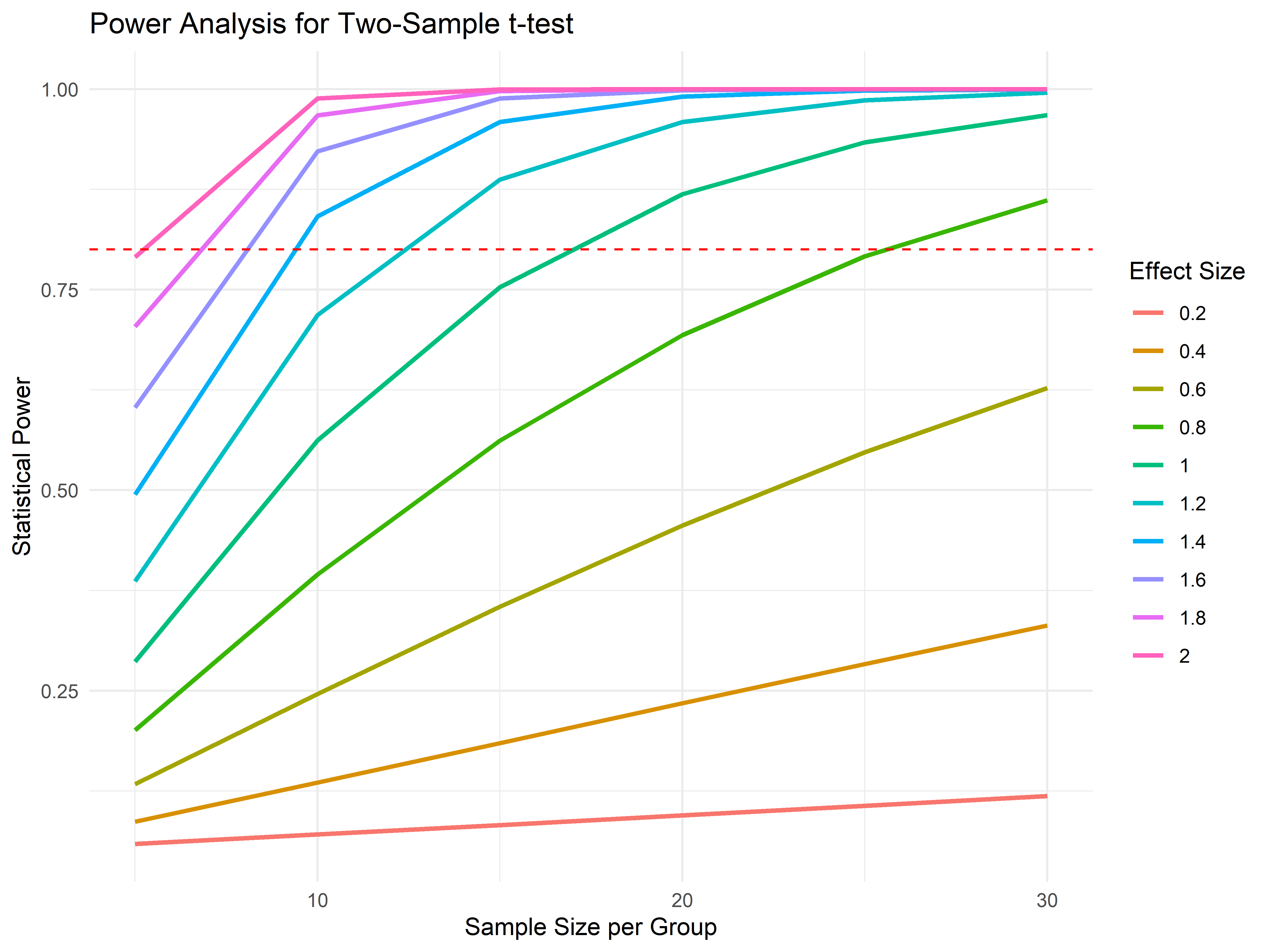
### Sample Size Calculation
```{r}
# Function for power analysis
calculate_power <- function(effect_size, sample_size_per_group, alpha = 0.05) {
  # Calculate power for two-sample t-test
  delta <- effect_size
  n <- sample_size_per_group

  # Non-centrality parameter
  ncp <- delta * sqrt(n/2)

  # Critical value
  t_crit <- qt(1 - alpha/2, df = 2*n - 2)

  # Power calculation
  power <- 1 - pt(t_crit, df = 2*n - 2, ncp = ncp) +
           pt(-t_crit, df = 2*n - 2, ncp = ncp)

  return(power)
}

# Power analysis for different effect sizes and sample sizes
effect_sizes <- seq(0.2, 2.0, by = 0.2)
sample_sizes <- seq(5, 30, by = 5)

power_results <- expand.grid(
  effect_size = effect_sizes,
  sample_size = sample_sizes
) %>%
  rowwise() %>%
  mutate(power = calculate_power(effect_size, sample_size))

# Visualize power analysis
ggplot(power_results, aes(x = sample_size, y = power, color = factor(effect_size))) +
  geom_line(size = 1) +
  geom_hline(yintercept = 0.8, linetype = "dashed", color = "red") +
  labs(title = "Power Analysis for Two-Sample t-test",
       x = "Sample Size per Group", y = "Statistical Power",
       color = "Effect Size") +
  theme_minimal()
```
## Summary
This chapter covered essential statistical methods for MS data analysis, including descriptive statistics, hypothesis testing, multivariate analysis, and clustering. It also connected those ideas to a real label-free proteomics case study using `DEP::UbiLength`, from a cleaned protein table through missingness-aware normalization, differential abundance testing, visualization, enrichment-ready output, and reproducible export.
## Exercises
1. **Design Matrices**: Given an experiment with two factors (Genotype: WT vs KO; Treatment: Ctrl vs Stim), write the R code to create a design matrix for a factorial analysis.
2. **Moderated t-tests**: Why is `limma`'s empirical Bayes moderation particularly valuable for mass spectrometry experiments with only 3–4 replicates per group?
3. **Visualization**: Using the results from the `UbiLength` case study, generate a volcano plot where features with a fold-change > 2 and adjusted p-value < 0.05 are highlighted in a different color.
4. **Multiple testing**: Re-run the case-study contrast and compare Benjamini–Hochberg, Benjamini–Yekutieli, and Bonferroni adjustment. How does the number of significant proteins change, and which is appropriate here?
5. **Blocking**: The design includes technical structure across sites. Show how you would use `limma::duplicateCorrelation()` to block on a subject/site variable, and contrast the result with the unblocked fit.
6. **Choose a differential abundance method**: For each of the three contrasting study designs below, select an appropriate differential abundance method from Section "Choosing a Differential Abundance Method" and defend your choice in 2–3 sentences: (a) TMT 10-plex with 5 vs 5 samples, no missing values; (b) Label-free DIA with 3 vs 3 samples, approximately 25% missing values; (c) Single-cell proteomics with 40 vs 40 cells, more than 60% missing values.
## Session Information
```{r}
sessionInfo()
```