# Audit Peptide-Spectrum Matches and Build an Identification Report
A database search engine returns a list of peptide–spectrum matches (PSMs) — candidate assignments of MS/MS spectra to peptide sequences. Not every PSM is correct. This chapter shows you how to load a PSM table into R, apply score-based FDR filtering with target–decoy statistics, flag common failure modes (shared peptides, missed cleavages, charge-state anomalies), and assemble a clean identification report that can be handed to quantification workflows.
::: {.callout-warning title="The One Mistake to Avoid"}
Filtering PSMs by a raw score threshold. A score cutoff gives you no control over the actual false-discovery rate. Always estimate FDR against decoy hits and filter to a target FDR instead.
:::
## Learning Objectives
By the end of this chapter you will be able to:
- Load a search-engine PSM table into R and understand its columns
- Apply score-based false-discovery-rate (FDR) filtering using target–decoy statistics
- Assess MS/MS spectrum quality before trusting an identification
- Diagnose common PSM failure modes: shared peptides, missed cleavages, charge-state anomalies, and contaminant hits
- Assemble a clean, quantification-ready identification report
## Setting Up Proteomics Environment
The R for Mass Spectrometry ecosystem provides specialized packages for proteomics analysis:
```{r}
library(Spectra)          # Core MS data structures
library(PSMatch)          # Peptide-spectrum matching
library(ProtGenerics)     # Generic functions for proteomics
library(QFeatures)        # Quantitative features handling
library(msdata)           # Example MS data
library(mzR)             # Reading raw MS data
library(dplyr)           # Data manipulation
library(ggplot2)         # Visualization
library(pheatmap)        # Heatmaps
library(limma)           # Statistical analysis
library(tidyverse)       # Data science tools
```
```{r}
# Load proteomics test data from msdata
proteomics_files <- msdata::proteomics(full.names = TRUE)
cat("Available proteomics files:\n")
for (i in seq_along(proteomics_files)) {
  cat(i, ":", basename(proteomics_files[i]), "\n")
}
# Select a file for analysis
selected_file <- proteomics_files[1]
cat("\nSelected file:", basename(selected_file), "\n")
```
## Understanding Proteomics Workflows
### Bottom-up Proteomics Pipeline
The typical bottom-up proteomics workflow involves:
1. **Sample preparation**: Protein extraction, digestion (usually with trypsin)
2. **LC-MS/MS analysis**: Liquid chromatography coupled to tandem mass spectrometry
3. **Database searching**: Matching MS/MS spectra to peptide sequences
4. **Protein inference**: Assembling peptides into protein identifications
5. **Quantitative analysis**: Comparing protein abundances across samples
```{mermaid}
%%| fig-width: 10
%%| fig-height: 8
flowchart TD
    subgraph Sample["Sample Preparation"]
        A[Protein Extraction] --> B[Reduction & Alkylation]
        B --> C[Enzymatic Digestion<br/>Trypsin]
        C --> D[Peptide Cleanup<br/>Desalting]
    end

    subgraph MS["LC-MS/MS Analysis"]
        D --> E[LC Separation<br/>Reverse Phase]
        E --> F[MS1 Scan<br/>Precursor Selection]
        F --> G[MS2 Fragmentation<br/>HCD/CID/ETD]
        G --> H[Raw Data<br/>mzML Files]
    end

    subgraph Search["Database Searching"]
        H --> I[Spectra Object<br/>R/Spectra]
        I --> J{Search Engine}
        J --> K1[Mascot]
        J --> K2[MaxQuant]
        J --> K3[MSFragger]
        K1 --> L[PSM Table<br/>PSMatch]
        K2 --> L
        K3 --> L
    end

    subgraph Inference["Protein Inference"]
        L --> M[Filter PSMs<br/>FDR < 1%]
        M --> N[Peptide Assembly<br/>Unique + Shared]
        N --> O[Protein Grouping<br/>Parsimony Principle]
    end

    subgraph Quant["Quantification"]
        O --> P{Quant Method?}
        P -->|Label-Free| Q1[XIC Integration<br/>MS1 Intensity]
        P -->|TMT/iTRAQ| Q2[Reporter Ions<br/>MS2 Intensity]
        P -->|SILAC| Q3[Heavy/Light Ratio<br/>MS1 Intensity]
        Q1 --> R[QFeatures Object]
        Q2 --> R
        Q3 --> R
    end

    subgraph Analysis["Statistical Analysis"]
        R --> S[PSM → Peptide<br/>Aggregation]
        S --> T[Peptide → Protein<br/>Summarization]
        T --> U[Differential Analysis<br/>limma/DEqMS]
        U --> V[Results<br/>Volcano/Heatmap]
    end

  style Sample fill:#D7E6FB,stroke:#27408B,stroke-width:3px,color:#102A43
  style MS fill:#FBE0FA,stroke:#B000B0,stroke-width:3px,color:#102A43
  style Search fill:#D7E6FB,stroke:#27408B,stroke-width:3px,color:#102A43
  style Inference fill:#FBE0FA,stroke:#B000B0,stroke-width:3px,color:#102A43
  style Quant fill:#D7E6FB,stroke:#27408B,stroke-width:3px,color:#102A43
  style Analysis fill:#FBE0FA,stroke:#B000B0,stroke-width:3px,color:#102A43
```
::: callout-important
## Key Proteomics Concepts
- **PSM (Peptide-Spectrum Match)**: One MS/MS spectrum matched to one peptide sequence
- **FDR (False Discovery Rate)**: Typically controlled at 1% using target-decoy approach
- **Protein Parsimony**: Minimal set of proteins explaining observed peptides
- **Missing Values**: Can occur at PSM, peptide, or protein level - handle appropriately
:::
### Data Structures in Proteomics
Proteomics data has a hierarchical structure: - **Spectra**: Raw MS and MS/MS data - **PSMs**: Peptide-Spectrum Matches from database search - **Peptides**: Unique peptide sequences - **Proteins**: Protein groups inferred from peptides
## MS/MS Spectral Data Processing
### Loading and Examining MS/MS Data
```{r}
# Load MS/MS data with error handling
tryCatch({
  ms_data <- Spectra(selected_file, backend = MsBackendMzR())
  ms_data <- setBackend(ms_data, backend = MsBackendDataFrame())
  cat("Successfully loaded real MS data\n")
}, error = function(e) {
  cat("Note: Using synthetic data due to mzR compatibility issues\n")
  cat("Error details:", conditionMessage(e), "\n\n")

  # Create synthetic MS/MS data
  set.seed(456)
  n_spectra <- 200

  library(S4Vectors)
  library(IRanges)

  # Generate peak data
  mz_list <- lapply(1:n_spectra, function(i) {
    sort(runif(sample(40:120, 1), 200, 1800))
  })

  intensity_list <- lapply(mz_list, function(mz_vals) {
    rlnorm(length(mz_vals), meanlog = 7, sdlog = 2)
  })

  # Generate MS levels (80% MS2, 20% MS1)
  ms_levels <- sample(1:2, n_spectra, replace = TRUE, prob = c(0.2, 0.8))

  # Create metadata DataFrame
  spd <- DataFrame(
    msLevel = ms_levels,
    rtime = seq(100, 4500, length.out = n_spectra),
    acquisitionNum = 1:n_spectra,
    precursorMz = ifelse(ms_levels == 1, NA_real_, runif(n_spectra, 400, 1600)),
    precursorCharge = ifelse(ms_levels == 1, NA_integer_, sample(2:4, n_spectra, replace = TRUE)),
    precursorIntensity = ifelse(ms_levels == 1, NA_real_, rlnorm(n_spectra, meanlog = 10, sdlog = 1.5)),
    collisionEnergy = ifelse(ms_levels == 1, NA_real_, runif(n_spectra, 25, 45)),
    polarity = rep(1L, n_spectra)
  )

  # Add peak data as list columns
  spd$mz <- NumericList(mz_list)
  spd$intensity <- NumericList(intensity_list)

  # Initialize backend and create Spectra object
  backend <- MsBackendDataFrame()
  backend <- backendInitialize(backend, spd)
  ms_data <<- Spectra(backend)
})
# Basic information about the data
cat("\nDataset summary:\n")
cat("Total spectra:", length(ms_data), "\n")
cat("MS levels:", paste(unique(msLevel(ms_data)), collapse = ", "), "\n")
cat("Scan range:", range(acquisitionNum(ms_data)), "\n")
cat("RT range:", round(range(rtime(ms_data)), 2), "seconds\n")
# MS2 spectra information
ms2_data <- filterMsLevel(ms_data, msLevel = 2)
cat("\nMS2 spectra:", length(ms2_data), "\n")
if (length(ms2_data) > 0) {
  cat("Precursor m/z range:", round(range(precursorMz(ms2_data), na.rm = TRUE), 2), "\n")
  cat("Charge state distribution:\n")
  print(table(precursorCharge(ms2_data)))
}
```
### MS/MS Spectrum Quality Assessment
```{r}
# Function to assess MS/MS spectrum quality
assess_ms2_quality <- function(ms2_spectra) {
  quality_metrics <- data.frame(
    spectrum_id = seq_along(ms2_spectra),
    precursor_mz = precursorMz(ms2_spectra),
    precursor_charge = precursorCharge(ms2_spectra),
    precursor_intensity = precursorIntensity(ms2_spectra),
    retention_time = rtime(ms2_spectra),
    total_ion_current = sapply(seq_along(ms2_spectra), function(i) {
      sum(intensity(ms2_spectra[i])[[1]], na.rm = TRUE)
    }),
    peak_count = sapply(seq_along(ms2_spectra), function(i) {
      length(intensity(ms2_spectra[i])[[1]])
    }),
    base_peak_intensity = sapply(seq_along(ms2_spectra), function(i) {
      max(intensity(ms2_spectra[i])[[1]], na.rm = TRUE)
    })
  )

  # Calculate signal-to-noise metrics
  quality_metrics$snr_estimate <- quality_metrics$base_peak_intensity /
                                  (quality_metrics$total_ion_current / quality_metrics$peak_count)

  return(quality_metrics)
}

# Assess quality for first 100 MS2 spectra
ms2_quality <- assess_ms2_quality(ms2_data[1:min(100, length(ms2_data))])

# Visualize quality metrics
quality_plots <- list()

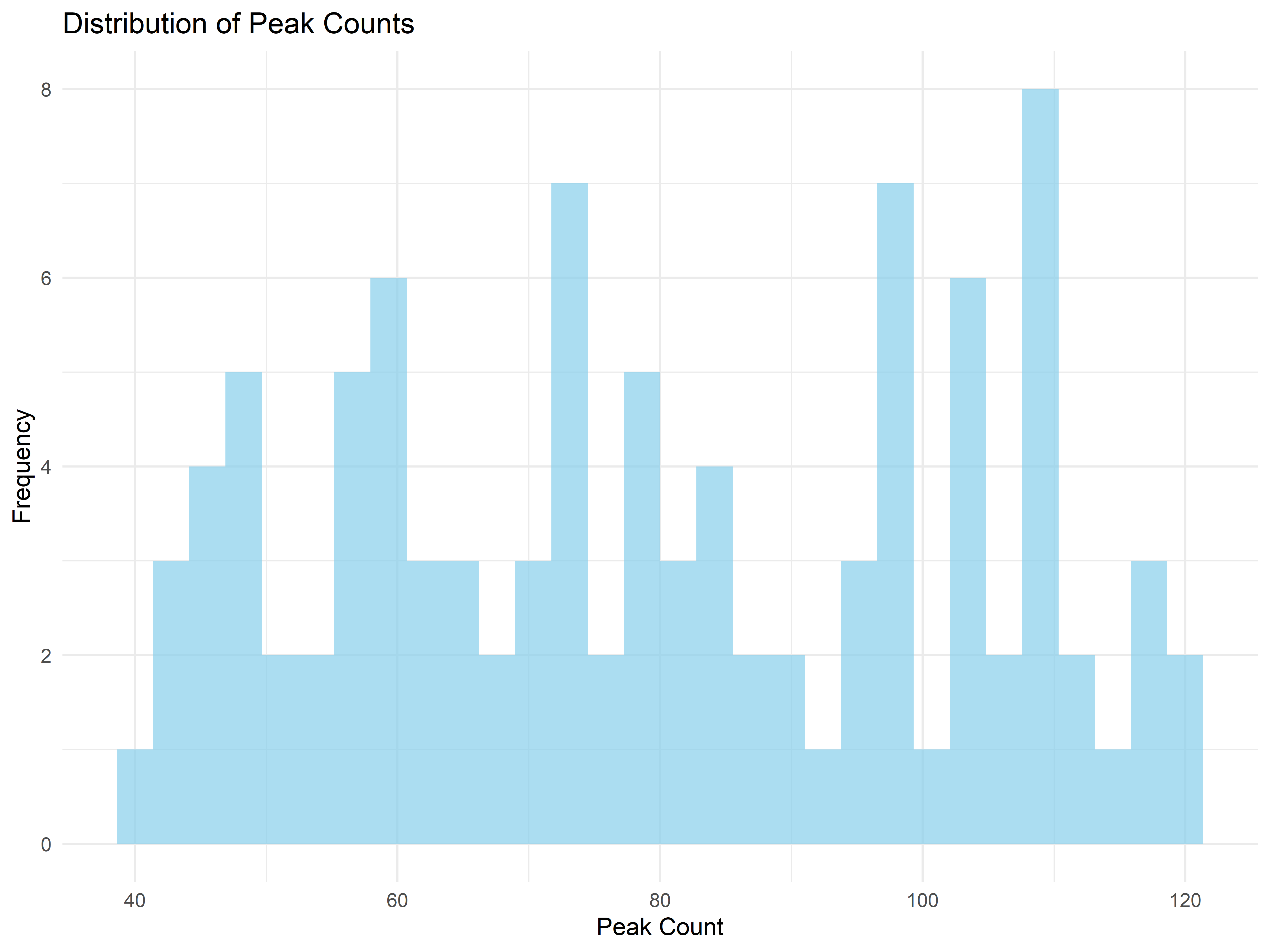
quality_plots[[1]] <- ggplot(ms2_quality, aes(x = peak_count)) +
  geom_histogram(bins = 30, fill = "skyblue", alpha = 0.7) +
  labs(title = "Distribution of Peak Counts", x = "Peak Count", y = "Frequency") +
  theme_minimal()

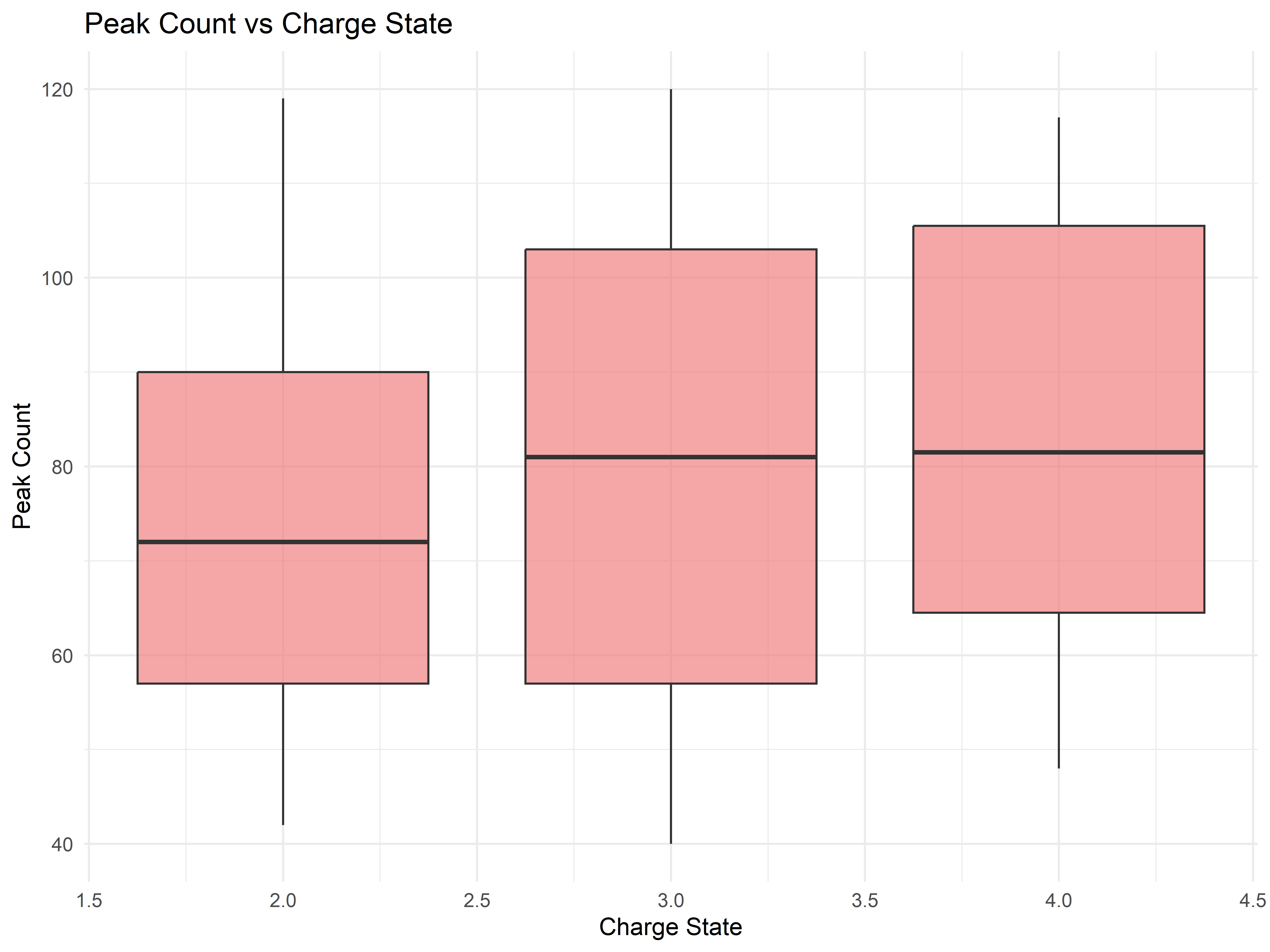
quality_plots[[2]] <- ggplot(ms2_quality, aes(x = precursor_charge, y = peak_count)) +
  geom_boxplot(aes(group = precursor_charge), fill = "lightcoral", alpha = 0.7) +
  labs(title = "Peak Count vs Charge State", x = "Charge State", y = "Peak Count") +
  theme_minimal()

# Print plots
print(quality_plots[[1]])
print(quality_plots[[2]])
```
### Spectrum Preprocessing
```{r}
# Function to preprocess MS/MS spectra
preprocess_ms2_spectrum <- function(spectrum_obj,
                                   min_intensity = 100,
                                   top_n_peaks = 150,
                                   remove_precursor = TRUE,
                                   precursor_tolerance = 1.5) {

  processed_spectra <- list()

  for (i in seq_along(spectrum_obj)) {
    mz_vals <- mz(spectrum_obj[i])[[1]]
    int_vals <- intensity(spectrum_obj[i])[[1]]
    precursor_mz_val <- precursorMz(spectrum_obj[i])

    if (length(mz_vals) == 0 || length(int_vals) == 0) {
      next
    }

    # Remove low-intensity peaks
    intensity_filter <- int_vals >= min_intensity
    mz_vals <- mz_vals[intensity_filter]
    int_vals <- int_vals[intensity_filter]

    # Remove precursor ion if requested
    if (remove_precursor && !is.na(precursor_mz_val)) {
      precursor_filter <- abs(mz_vals - precursor_mz_val) > precursor_tolerance
      mz_vals <- mz_vals[precursor_filter]
      int_vals <- int_vals[precursor_filter]
    }

    # Keep only top N peaks
    if (length(int_vals) > top_n_peaks) {
      top_indices <- order(int_vals, decreasing = TRUE)[1:top_n_peaks]
      mz_vals <- mz_vals[top_indices]
      int_vals <- int_vals[top_indices]

      # Re-order by m/z
      order_indices <- order(mz_vals)
      mz_vals <- mz_vals[order_indices]
      int_vals <- int_vals[order_indices]
    }

    # Normalize intensities
    int_vals <- int_vals / max(int_vals) * 100

    processed_spectra[[i]] <- list(
      spectrum_index = i,
      mz = mz_vals,
      intensity = int_vals,
      precursor_mz = precursor_mz_val,
      precursor_charge = precursorCharge(spectrum_obj[i]),
      retention_time = rtime(spectrum_obj[i]),
      original_peak_count = length(intensity(spectrum_obj[i])[[1]]),
      processed_peak_count = length(int_vals)
    )
  }

  return(processed_spectra)
}

# Preprocess first 50 MS2 spectra
processed_ms2 <- preprocess_ms2_spectrum(ms2_data[1:50])

# Remove NULL entries
processed_ms2 <- processed_ms2[!sapply(processed_ms2, is.null)]

cat("Processed", length(processed_ms2), "MS/MS spectra\n")
# Example: visualize a processed spectrum
if (length(processed_ms2) > 0) {
  example_spectrum <- processed_ms2[[1]]

  spectrum_df <- data.frame(
    mz = example_spectrum$mz,
    intensity = example_spectrum$intensity
  )

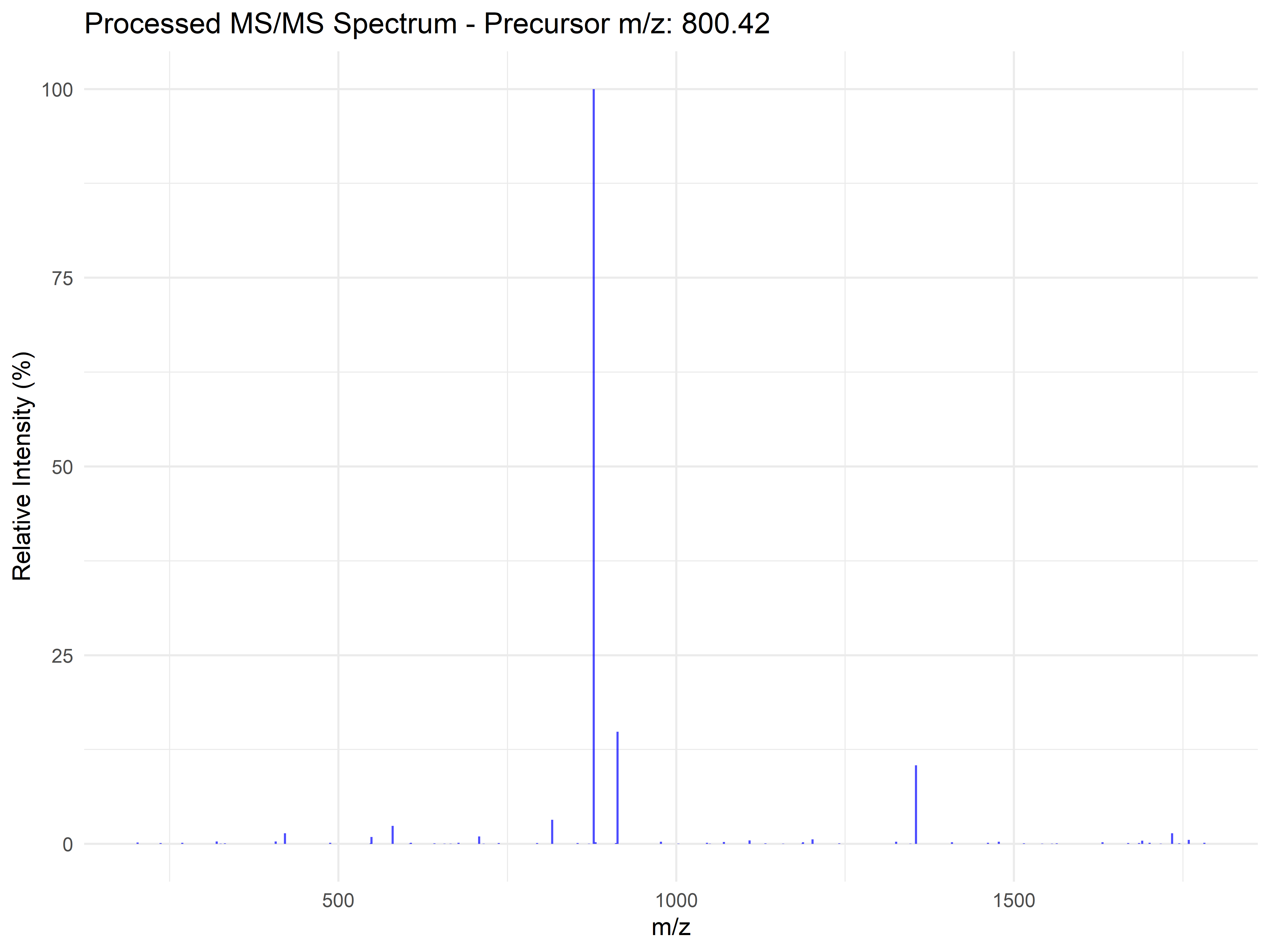
  ggplot(spectrum_df, aes(x = mz, y = intensity)) +
    geom_segment(aes(xend = mz, yend = 0), color = "blue", alpha = 0.7) +
    labs(title = paste("Processed MS/MS Spectrum - Precursor m/z:",
                      round(example_spectrum$precursor_mz, 2)),
         x = "m/z", y = "Relative Intensity (%)") +
    theme_minimal()
}
```
## Protein Identification
### Peptide Spectral Matching
```{r}
# Simulate protein database and peptide identification results
create_protein_database <- function() {
  # Create a simplified protein database
  proteins <- data.frame(
    protein_id = paste0("PROT_", 1:100),
    protein_name = paste0("Protein_", 1:100),
    gene_name = paste0("GENE_", 1:100),
    organism = "Homo sapiens",
    sequence_length = sample(100:2000, 100),
    stringsAsFactors = FALSE
  )

  # Generate theoretical peptides for each protein
  peptide_db <- data.frame()
  peptide_counter <- 1

  for (i in 1:nrow(proteins)) {
    # Simulate 5-15 peptides per protein
    n_peptides <- sample(5:15, 1)

    for (j in 1:n_peptides) {
      # Generate random peptide sequence (simplified)
      aa_codes <- c("A", "R", "N", "D", "C", "E", "Q", "G", "H", "I",
                   "L", "K", "M", "F", "P", "S", "T", "W", "Y", "V")
      peptide_length <- sample(7:25, 1)
      sequence <- paste(sample(aa_codes, peptide_length, replace = TRUE), collapse = "")

      # Calculate theoretical m/z (simplified calculation)
      theoretical_mass <- peptide_length * 110  # Rough average AA mass
      charge <- sample(2:4, 1)
      theoretical_mz <- (theoretical_mass + charge * 1.007276) / charge

      peptide_db <- rbind(peptide_db, data.frame(
        peptide_id = paste0("PEP_", sprintf("%04d", peptide_counter)),
        protein_id = proteins$protein_id[i],
        sequence = sequence,
        theoretical_mz = theoretical_mz,
        charge = charge,
        peptide_counter = peptide_counter
      ))

      peptide_counter <- peptide_counter + 1
    }
  }

  return(list(proteins = proteins, peptides = peptide_db))
}

db_info <- create_protein_database()
cat("Created database with", nrow(db_info$proteins), "proteins and",
    nrow(db_info$peptides), "peptides\n")
```
### Simulate Peptide-Spectrum Matches (PSMs)
```{r}
# Simulate PSM results
simulate_psm_results <- function(processed_spectra, peptide_db, match_probability = 0.3) {
  psm_results <- data.frame()

  for (i in seq_along(processed_spectra)) {
    spectrum <- processed_spectra[[i]]

    # Simulate whether this spectrum gets identified
    if (runif(1) < match_probability) {
      # Find potential peptide matches based on precursor m/z
      mz_tolerance <- 0.01  # 10 ppm at m/z 1000

      potential_matches <- which(
        abs(peptide_db$theoretical_mz - spectrum$precursor_mz) < mz_tolerance &
        peptide_db$charge == spectrum$precursor_charge
      )

      if (length(potential_matches) > 0) {
        # Select best match (random for simulation)
        best_match <- sample(potential_matches, 1)

        # Simulate scoring metrics
        xcorr_score <- runif(1, 1.5, 4.5)
        delta_cn <- runif(1, 0.1, 0.8)
        sp_score <- sample(200:800, 1)
        mass_error_ppm <- runif(1, -5, 5)

        # Calculate q-value based on score (simplified)
        q_value <- 1 / (1 + exp((xcorr_score - 2) * 3))  # Sigmoid function

        psm_results <- rbind(psm_results, data.frame(
          spectrum_index = i,
          scan_number = i,
          peptide_id = peptide_db$peptide_id[best_match],
          protein_id = peptide_db$protein_id[best_match],
          sequence = peptide_db$sequence[best_match],
          charge = spectrum$precursor_charge,
          theoretical_mz = peptide_db$theoretical_mz[best_match],
          observed_mz = spectrum$precursor_mz,
          mass_error_ppm = mass_error_ppm,
          retention_time = spectrum$retention_time,
          xcorr = xcorr_score,
          delta_cn = delta_cn,
          sp_score = sp_score,
          q_value = q_value
        ))
      }
    }
  }

  return(psm_results)
}

# Generate PSM results
psm_results <- simulate_psm_results(processed_ms2, db_info$peptides)
cat("Generated", nrow(psm_results), "PSMs\n")
if (nrow(psm_results) > 0) {
  head(psm_results)
}
```
### PSM Quality Assessment and Filtering
```{r}
# Assess PSM quality
assess_psm_quality <- function(psm_data) {
  # Quality distribution plots
  quality_plots <- list()

  # XCorr distribution
  quality_plots[[1]] <- ggplot(psm_data, aes(x = xcorr)) +
    geom_histogram(bins = 30, fill = "lightblue", alpha = 0.7) +
    labs(title = "XCorr Score Distribution", x = "XCorr", y = "Count") +
    theme_minimal()

  # q-value distribution
  quality_plots[[2]] <- ggplot(psm_data, aes(x = q_value)) +
    geom_histogram(bins = 30, fill = "lightcoral", alpha = 0.7) +
    scale_x_log10() +
    labs(title = "Q-value Distribution", x = "Q-value (log10)", y = "Count") +
    theme_minimal()

  # Mass error distribution
  quality_plots[[3]] <- ggplot(psm_data, aes(x = mass_error_ppm)) +
    geom_histogram(bins = 30, fill = "lightgreen", alpha = 0.7) +
    labs(title = "Mass Error Distribution", x = "Mass Error (ppm)", y = "Count") +
    theme_minimal()

  return(quality_plots)
}

if (nrow(psm_results) > 0) {
  quality_plots <- assess_psm_quality(psm_results)
  print(quality_plots[[1]])
  print(quality_plots[[2]])
  print(quality_plots[[3]])
}
```
### The Target–Decoy FDR Framework
Before writing any filter code, you must understand how the false discovery rate is actually estimated in proteomics. Database search engines do not know which PSMs are correct — they only produce scores. The target–decoy strategy solves this with a simple but powerful idea:
1. **Concatenate your real protein database with a decoy database** — reversed or shuffled sequences that cannot exist in nature.
2. **Search against the combined database.** Every PSM either matches a target (real) or a decoy (fake) sequence.
3. **Count decoy matches as false positives.** Because decoys are biologically impossible, any PSM assigned to a decoy must be incorrect. Assuming false positives are equally likely among target and decoy matches:
$$\text{FDR} = \frac{\text{Number of decoy PSMs above score threshold}}{\text{Number of target PSMs above score threshold}}$$
This gives you the **PSM-level FDR** — the expected proportion of incorrect identifications among all PSMs that pass the score cutoff. The standard threshold is **1 % FDR** at the PSM level.
**The PSM-to-protein FDR gap.** A critical and frequently overlooked point: controlling FDR at 1 % at the PSM level does **not** guarantee 1 % FDR at the protein level. If a false PSM maps to a protein with no other evidence, that protein becomes a false identification. Conversely, if many true PSMs map to one protein, a single false PSM among them may not change the protein call. Protein-level FDR must be estimated separately — typically by applying the same target–decoy logic at the protein-group level, or by using a picked-protein FDR strategy (Savitski et al., 2015).
**In practice:**
- PSM-level FDR ≤ 1 % — the minimum standard for publication
- Peptide-level FDR ≤ 1 % — stricter, requires at least 2 PSMs per peptide
- Protein-level FDR ≤ 1 % — the gold standard; proteins with only one peptide ("one-hit wonders") are the most vulnerable to false discovery
### PSM Filtering and FDR Control
```{r}
# Apply PSM filters
filter_psms <- function(psm_data,
                       xcorr_threshold = 2.0,
                       qvalue_threshold = 0.01,
                       mass_error_threshold = 10) {

  # Apply filters
  filtered_psms <- psm_data %>%
    filter(
      xcorr >= xcorr_threshold,
      q_value <= qvalue_threshold,
      abs(mass_error_ppm) <= mass_error_threshold
    )

  cat("PSM filtering results:\n")
  cat("  Original PSMs:", nrow(psm_data), "\n")
  cat("  XCorr filter (>=", xcorr_threshold, "):",
      sum(psm_data$xcorr >= xcorr_threshold), "\n")
  cat("  Q-value filter (<=", qvalue_threshold, "):",
      sum(psm_data$q_value <= qvalue_threshold), "\n")
  cat("  Mass error filter (<=", mass_error_threshold, "ppm):",
      sum(abs(psm_data$mass_error_ppm) <= mass_error_threshold), "\n")
  cat("  Final filtered PSMs:", nrow(filtered_psms), "\n")
  cat("  PSM-level FDR:", round(mean(filtered_psms$q_value) * 100, 2), "%\n")

  return(filtered_psms)
}

if (nrow(psm_results) > 0) {
  filtered_psms <- filter_psms(psm_results)
}
```
## Protein Inference and Quantification
### Protein Grouping
```{r}
# Perform protein inference
protein_inference <- function(filtered_psms, protein_db) {
  if (nrow(filtered_psms) == 0) {
    return(data.frame())
  }

  # Group PSMs by protein
  protein_groups <- filtered_psms %>%
    group_by(protein_id) %>%
    summarise(
      peptide_count = n_distinct(sequence),
      psm_count = n(),
      unique_peptide_count = n_distinct(sequence),  # Simplified - assume all peptides are unique
      sequence_coverage = peptide_count * 10,  # Rough estimate
      best_xcorr = max(xcorr),
      mean_mass_error = mean(mass_error_ppm),
      .groups = 'drop'
    ) %>%
    filter(peptide_count >= 2)  # Require at least 2 peptides

  # Add protein information
  protein_groups <- protein_groups %>%
    left_join(protein_db, by = "protein_id")

  return(protein_groups)
}

if (exists("filtered_psms") && nrow(filtered_psms) > 0) {
  protein_groups <- protein_inference(filtered_psms, db_info$proteins)
  cat("Identified", nrow(protein_groups), "protein groups\n")

  if (nrow(protein_groups) > 0) {
    head(protein_groups)
  }
}
```
### Label-Free Quantification
```{r}
# Simulate label-free quantification data
simulate_lfq_data <- function(protein_groups, n_samples = 12) {
  if (nrow(protein_groups) == 0) {
    return(list())
  }

  # Create sample information
  sample_info <- data.frame(
    sample_id = paste0("Sample_", 1:n_samples),
    condition = rep(c("Control", "Treatment"), each = n_samples/2),
    batch = rep(1:3, each = n_samples/3),
    injection_order = 1:n_samples
  )

  # Create intensity matrix
  intensity_matrix <- matrix(0, nrow = nrow(protein_groups), ncol = n_samples)
  rownames(intensity_matrix) <- protein_groups$protein_id
  colnames(intensity_matrix) <- sample_info$sample_id

  # Simulate protein abundances
  for (i in 1:nrow(protein_groups)) {
    base_abundance <- rlnorm(1, meanlog = 20, sdlog = 2)

    for (j in 1:n_samples) {
      # Add condition effect for some proteins
      condition_effect <- ifelse(sample_info$condition[j] == "Treatment" &
                                i <= nrow(protein_groups) * 0.2,
                                log2(1.5), 0)  # 1.5-fold change for 20% of proteins

      # Add batch effect
      batch_effect <- rnorm(1, 0, 0.1) * sample_info$batch[j]

      # Add biological and technical variation
      log_intensity <- log2(base_abundance) + condition_effect + batch_effect + rnorm(1, 0, 0.3)

      # Convert back to linear scale with some probability of missing values
      if (runif(1) > 0.1) {  # 90% detection rate
        intensity_matrix[i, j] <- 2^log_intensity
      }
    }
  }

  # Convert zero values to NA
  intensity_matrix[intensity_matrix == 0] <- NA

  return(list(
    intensity_matrix = intensity_matrix,
    sample_info = sample_info,
    protein_info = protein_groups
  ))
}

if (exists("protein_groups") && nrow(protein_groups) > 0) {
  lfq_data <- simulate_lfq_data(protein_groups)

  cat("Created LFQ dataset:\n")
  cat("  Proteins:", nrow(lfq_data$intensity_matrix), "\n")
  cat("  Samples:", ncol(lfq_data$intensity_matrix), "\n")
  cat("  Missing values:",
      round(sum(is.na(lfq_data$intensity_matrix)) / length(lfq_data$intensity_matrix) * 100, 1), "%\n")
}
```
### Data Normalization and Preprocessing
```{r}
# Normalize proteomics data
normalize_proteomics_data <- function(intensity_matrix, method = "median") {
  log_matrix <- log2(intensity_matrix)

  if (method == "median") {
    # Median normalization
    sample_medians <- apply(log_matrix, 2, median, na.rm = TRUE)
    global_median <- median(sample_medians, na.rm = TRUE)
    normalization_factors <- global_median - sample_medians

    for (i in 1:ncol(log_matrix)) {
      log_matrix[, i] <- log_matrix[, i] + normalization_factors[i]
    }

  } else if (method == "quantile") {
    # Quantile normalization (simplified)
    for (i in 1:ncol(log_matrix)) {
      log_matrix[, i] <- scale(log_matrix[, i])[, 1]
    }
  }

  return(2^log_matrix)  # Convert back to linear scale
}

if (exists("lfq_data")) {
  # Normalize data
  normalized_intensities <- normalize_proteomics_data(lfq_data$intensity_matrix)

  # Visualize normalization effect
  # Before normalization
  sample_medians_before <- apply(log2(lfq_data$intensity_matrix), 2, median, na.rm = TRUE)
  sample_medians_after <- apply(log2(normalized_intensities), 2, median, na.rm = TRUE)

  normalization_df <- data.frame(
    sample = rep(colnames(lfq_data$intensity_matrix), 2),
    median_intensity = c(sample_medians_before, sample_medians_after),
    normalization = rep(c("Before", "After"), each = length(sample_medians_before))
  )

  ggplot(normalization_df, aes(x = sample, y = median_intensity, fill = normalization)) +
    geom_bar(stat = "identity", position = "dodge", alpha = 0.7) +
    labs(title = "Effect of Median Normalization",
         x = "Sample", y = "Median log2 Intensity",
         fill = "Normalization") +
    theme_minimal() +
    theme(axis.text.x = element_text(angle = 45, hjust = 1))
}
```
## Differential Expression Analysis
### Statistical Testing with limma
```{r}
# Perform differential expression analysis
perform_limma_analysis <- function(intensity_matrix, sample_info) {
  # Convert to log2 scale
  log_matrix <- log2(intensity_matrix)

  # Create design matrix
  condition <- factor(sample_info$condition)
  batch <- factor(sample_info$batch)
  design <- model.matrix(~ 0 + condition + batch)
  colnames(design)[1:2] <- levels(condition)

  # Fit linear model
  fit <- lmFit(log_matrix, design)

  # Create contrast matrix
  contrast_matrix <- makeContrasts(
    TreatmentVsControl = Treatment - Control,
    levels = design
  )

  # Apply contrasts
  fit2 <- contrasts.fit(fit, contrast_matrix)
  fit2 <- eBayes(fit2)

  # Extract results
  results <- topTable(fit2, coef = "TreatmentVsControl",
                     number = Inf, adjust.method = "BH")

  return(list(fit = fit2, results = results))
}

if (exists("normalized_intensities")) {
  limma_results <- perform_limma_analysis(normalized_intensities, lfq_data$sample_info)

  cat("Differential expression results:\n")
  cat("  Significant proteins (p < 0.05):",
      sum(limma_results$results$P.Value < 0.05, na.rm = TRUE), "\n")
  cat("  Significant proteins (FDR < 0.05):",
      sum(limma_results$results$adj.P.Val < 0.05, na.rm = TRUE), "\n")

  head(limma_results$results)
}
```
### Volcano Plot
```{r}
# Create volcano plot
if (exists("limma_results")) {
  volcano_data <- limma_results$results %>%
    mutate(
      protein_id = rownames(.),
      significant = adj.P.Val < 0.05 & abs(logFC) > log2(1.2),
      direction = case_when(
        logFC > log2(1.2) & adj.P.Val < 0.05 ~ "Up",
        logFC < -log2(1.2) & adj.P.Val < 0.05 ~ "Down",
        TRUE ~ "NS"
      )
    )

  ggplot(volcano_data, aes(x = logFC, y = -log10(P.Value))) +
    geom_point(aes(color = direction), alpha = 0.7) +
    scale_color_manual(values = c("Up" = "red", "Down" = "blue", "NS" = "gray")) +
    geom_hline(yintercept = -log10(0.05), linetype = "dashed") +
    geom_vline(xintercept = c(-log2(1.2), log2(1.2)), linetype = "dashed") +
    labs(title = "Volcano Plot - Proteomics Differential Expression",
         x = "log2 Fold Change", y = "-log10 P-value",
         color = "Regulation") +
    theme_minimal()
}
```
### Protein Set Analysis
```{r}
# Simulate gene ontology enrichment
simulate_go_enrichment <- function(significant_proteins, all_proteins) {
  # Create mock GO terms
  go_terms <- c("Protein Binding", "Metabolic Process", "Transport",
                "Cell Division", "DNA Repair", "Signal Transduction")

  enrichment_results <- data.frame()

  for (go_term in go_terms) {
    # Randomly assign proteins to GO terms
    go_proteins <- sample(all_proteins, size = sample(20:100, 1))

    # Calculate overlap with significant proteins
    overlap <- intersect(significant_proteins, go_proteins)

    # Fisher's exact test
    contingency <- matrix(c(
      length(overlap),
      length(significant_proteins) - length(overlap),
      length(go_proteins) - length(overlap),
      length(all_proteins) - length(significant_proteins) -
        length(go_proteins) + length(overlap)
    ), nrow = 2)

    fisher_result <- fisher.test(contingency, alternative = "greater")

    enrichment_results <- rbind(enrichment_results, data.frame(
      go_term = go_term,
      overlap_size = length(overlap),
      go_size = length(go_proteins),
      p_value = fisher_result$p.value,
      odds_ratio = fisher_result$estimate
    ))
  }

  enrichment_results$adj_p_value <- p.adjust(enrichment_results$p_value, method = "BH")
  return(enrichment_results[order(enrichment_results$p_value), ])
}

if (exists("volcano_data")) {
  significant_proteins <- volcano_data$protein_id[volcano_data$significant]
  all_proteins <- volcano_data$protein_id

  if (length(significant_proteins) > 0) {
    go_results <- simulate_go_enrichment(significant_proteins, all_proteins)

    cat("GO enrichment analysis:\n")
    print(go_results)

    # Plot enrichment results
    ggplot(go_results, aes(x = reorder(go_term, -log10(p_value)),
                          y = -log10(p_value))) +
      geom_bar(stat = "identity", fill = "steelblue", alpha = 0.7) +
      geom_hline(yintercept = -log10(0.05), linetype = "dashed", color = "red") +
      coord_flip() +
      labs(title = "GO Term Enrichment Analysis",
           x = "GO Term", y = "-log10 P-value") +
      theme_minimal()
  }
}
```
## Data Visualization and Reporting
### Heat Map of Significant Proteins
```{r}
# Create heat map for significant proteins
if (exists("volcano_data") && exists("normalized_intensities")) {
  significant_proteins <- volcano_data$protein_id[volcano_data$significant]

  if (length(significant_proteins) > 5) {  # Need at least 5 proteins for meaningful heatmap
    # Select top significant proteins
    top_proteins <- head(significant_proteins, 20)
    heatmap_data <- log2(normalized_intensities[top_proteins, ])

    # Create sample annotation
    annotation_col <- data.frame(
      Condition = lfq_data$sample_info$condition,
      Batch = factor(lfq_data$sample_info$batch),
      row.names = lfq_data$sample_info$sample_id
    )

    # Generate heat map
    pheatmap(heatmap_data,
             annotation_col = annotation_col,
             scale = "row",
             clustering_distance_rows = "euclidean",
             clustering_distance_cols = "euclidean",
             show_rownames = TRUE,
             show_colnames = TRUE,
             main = "Heat Map of Significantly Changed Proteins")
  }
}
```
## Exercises
1. Analyze real proteomics data from a public repository
2. Implement different protein inference algorithms
3. Compare various normalization methods for label-free quantification
4. Perform time-course proteomics analysis
5. Integrate proteomics with other omics data types
## Summary
This chapter covered comprehensive proteomics data analysis workflows, including MS/MS data processing, protein identification, quantification, and differential expression analysis. These methods are essential for extracting biological insights from bottom-up proteomics experiments.
## Session Information
```{r}
sessionInfo()
```